library(tidyverse)
library(MASS)
library(ggplot2)
library(glmnet)
library(hdm)
library(AER)Bias Simulation
Introduction
In this walkthrough we will run through a simulation that has been used in Fitzgerald Sice et al. (2023) which will help us understand when causal inference regressions (like Lasso and Double Robust Lasso) work and when they do not.
Reading:
Fitzgerald Sice, Jack and Lattimore, Finnian and Robinson, Tim and Zhu, Anna, Practical Insights Into Applying Double LASSO (May 18, 2023). Available at SSRN: https://ssrn.com/abstract=4452778 or http://dx.doi.org/10.2139/ssrn.4452778
The Background
Consider a model of the following form
\[\begin{equation} y_i = \delta D_i + \mathbf{x}_i\mathbf{\beta}_1 + \beta_2~u_i+ \epsilon_i \end{equation}\]
where the variables represent
- an outcome variable of interest, \(y_i\), for individual \(i\)
- a treatment variable, \(D_i\), which represents whether individual received some treatment (\(D_i=1\)) or not (\(D_i=1\))
- a vector of observable covariates associated to individual \(i\), \(\mathbf{x}_i\), where this includes a constant.
- a vector of unobservable covariates associated to individual \(i\), \(\mathbf{u}_i\).
In addition to this we consider a third category of variables, instruments \(\mathbf{z_i}\), these are variables that are observable, are excluded from the above model for \(y_i\), but have explanatory power for the treatment variable as per
\[\begin{equation} d_i = \mathbf{x}_i\mathbf{\beta}_3 + \beta_4~u_i + \gamma~z_i + \nu_i \end{equation}\]
Below we will simulate data from such a setup and establish how different regression approaches perform, always aiming to obtain a good estimate of the parameter capturing the treatment effect of \(D\) on \(y\), here the parameter \(\delta\).
The estimation methods we will apply are the
- The Post LASSO (forcing \(D_i\) to be included in the LASSO process)
- The Post Lasso adding \(D_i\) after unconstrained variable selection through LASSO
- The Post Double Selection LASSO
Inthis workthrough we will not go in detail through the different methods. If you are interested you can work through the workthroughs on Ridge and LASSO and Post Double Selection LASSO on the ECLR webpage.
Simulation Setup
We begin to introduce the data generating process (DGP) that is the basis of the simulation in the Fitzferald Sice paper. Later we shall introduce different setups.
No unobservables - No instruments
We begin with the situation in which there are no relevant unobservable variables, meaning we set \(\beta_2=\gamma=0\) which simplifies the data generating process significantly and none of the included variables are instruments
\[\begin{eqnarray} y_i &=& \delta D_i + \mathbf{x}_i\mathbf{\beta}_1 + \epsilon_i\\ d_i &=& \mathbf{x}_i\mathbf{\beta}_3 + \nu_i \end{eqnarray}\]
We write a function for the DGP whcih we will then later reuse inside a loop for the simulation.
We begin by simulating the error terms coming from standard normal distributions.
dgp1 <- function(n){
    # Simulates Fitzgerald Sice et al
    #  DGP from Section 3.1
    #   d = x * beta_3 + nu
    #   y = delta D + x * beta_1 + epsilon

    eps <- rnorm(n)
    nu <- rnorm(n)

    # Simulates j = 200 variables of X ~ N(0, Sigma)
    J = 200
    mu = rep(0, J)# mean is 0 for all j
    rho <- 0.5  # Define the decay factor FOR CORR MATRIX
    first_row <- rho^(0:(J - 1))
    Sigma <- toeplitz(first_row)   # Generate the covariance matrix using toeplitz
    x <- mvrnorm(n, mu, Sigma)

    # parameters
    c1 <- 0.3
    c3 <- 0.8
    delta <- 0.5
    beta0 <- 1/(seq(1,J,1)^2)
    beta0 <- as.matrix(beta0, J, 1)
    beta1 <- c1 * beta0
    beta3 <- c3 * beta0

    # generate d and y
    d <- x %*% beta3 + nu
    y <- delta*d + x %*% beta1 + eps
    return(list(y,d,x))
}

data <- dgp1(1000)
ysim <- unlist(data[[1]])
dsim <- unlist(data[[2]])
xsim <- unlist(data[[3]])

Regy <- summary(lm(ysim~., data.frame(ysim,xsim)))
Regd <- summary(lm(dsim~., data.frame(dsim,xsim)))
paste("R^2 in y equation =", Regy$r.squared)
[1] "R^2 in y equation = 0.521009361070768"paste("R^2 in d equation =", Regd$r.squared)[1] "R^2 in d equation = 0.591651676262392"Let’s see what values of \(R^2_y\) and \(R^2_d\) we get for these settings of c1 and c3. \(R^2_y\) and \(R^2_d\) are the \(R^2\) from the reduced form regressions of \(y\) (or \(d\)) on the variables in \(x\). In the paper they use a sample size of \(n = 100\) and \(J=200\) variables. This means that we cannot calculate \(R^2\) from such a regression. For the simulation below we therefore use \(n=1000\).
nsim =  50  # don't need many sims ot get an idea

save_R2 <- matrix(NA,nrow = nsim, ncol = 2)

for (i in 1:nsim){
  data <- dgp1(1000)
  ysim <- unlist(data[[1]])
  dsim <- unlist(data[[2]])
  xsim <- unlist(data[[3]])

  Regy <- summary(lm(ysim~., data.frame(ysim,xsim)))
  Regd <- summary(lm(dsim~., data.frame(dsim,xsim)))
  save_R2[i,1] <- Regy$r.squared
  save_R2[i,2] <- Regd$r.squared
  #print(paste("R^2 in y equation =", Regy$r.squared, ",R^2 in d equation =", Regd$r.squared))

}
Now we can plot the distribution for the two reduced form \(R^2\)s.
save_R2 <- as.data.frame(save_R2) %>% rename(R2y = V1, R2d = V2)
#create long dataframe, better for plotting
save_R2 <- save_R2 %>% pivot_longer(everything(),names_to = "type", values_to = "R2")

plot_den_R2 <- ggplot(save_R2, aes(x = R2, colour = type, fill = type)) +
  geom_density(alpha = .3, size = 1) +
  labs(title = "Distribution of reduced form R2")
Warning: Using `size` aesthetic for lines was deprecated in ggplot2 3.4.0.
ℹ Please use `linewidth` instead.plot_den_R2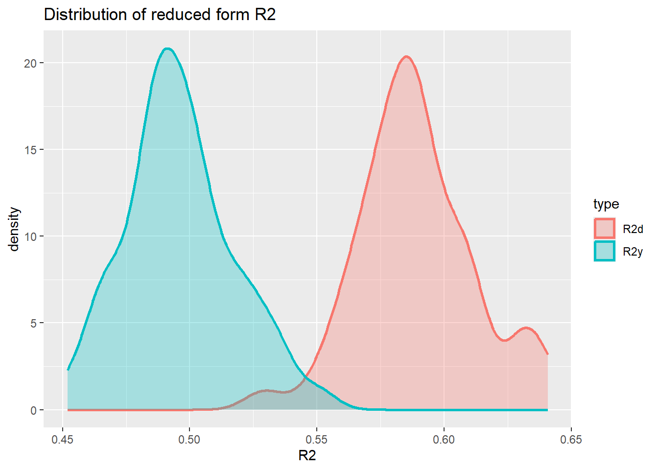
Varying the c1 and c3 parameters in the simulation will change these distributions. However, it appears impossible to achieve \(R^2_d = 0.8\) and \(R^2_y = 0.2\).
Estimation Strategies
We shall now proceed with implementing the different estimation strategies in this context. We simulate the above process 500 times, each simulation simulating \(n=100\) observations. As we are using \(J=200\) covariates (\(x\)) we cannot run a regression straight but we do have to apply reduction techniques.
- The Post LASSO (forcing \(D_i\) to be included in the LASSO process), fPSL
- The Post Lasso adding \(D_i\) after unconstrained variable selection through LASSO, PSL
- The Post Double Selection LASSO, PDL
Let’s first simulate one process and apply the methods.
set.seed(1)

data <- dgp1(100)
y.sim <- unlist(data[[1]])
colnames(y.sim) <- "Y"
d.sim <- unlist(data[[2]])
colnames(d.sim) <- "D"
x.sim <- unlist(data[[3]])
colnames(x.sim) <- paste0("X", 1:200)
dx.sim <- cbind(d.sim,x.sim)
colnames(dx.sim) <- c("D",paste0("X", 1:200))
fPSL
Let’s start with the simple post LASSO regression where D is part of the variables for selection.
cv_lasso=cv.glmnet(dx.sim,y.sim,family="gaussian",nfolds=10,alpha=1)
lasso.coef.lambda.1se <- as.matrix(coef(cv_lasso, s = "lambda.1se"))

# Now need to pick the selected variables
sel_vars <- rownames(lasso.coef.lambda.1se)[lasso.coef.lambda.1se > 0.0]
print(sel_vars)
[1] "(Intercept)" "D" "X1" # Now run post LASSO regression
sel_vars <- sel_vars[sel_vars != "(Intercept)"] # removes the intercept
pL.data <- data.frame(Y = y.sim, dx.sim[, colnames(dx.sim) %in% sel_vars])
pL.reg <- lm(Y~., data = pL.data)
summary(pL.reg)
Call:
lm(formula = Y ~ ., data = pL.data)

Residuals:
    Min      1Q  Median      3Q     Max
-2.3692 -0.6011 -0.0492  0.5867  2.4501

Coefficients:
            Estimate Std. Error t value Pr(>|t|)
(Intercept)  0.11582    0.09113   1.271  0.20677
D            0.52495    0.09128   5.751 1.03e-07 ***
X1           0.29978    0.10863   2.760  0.00692 **
---
Signif. codes:  0 '***' 0.001 '**' 0.01 '*' 0.05 '.' 0.1 ' ' 1

Residual standard error: 0.9109 on 97 degrees of freedom
Multiple R-squared:  0.5553,    Adjusted R-squared:  0.5461
F-statistic: 60.56 on 2 and 97 DF,  p-value: < 2.2e-16
You can see here that the coefficient to D is very small (compared to the true \(\alpha =0.5\)).
In the way we implemented this above it is actually possible that the D variable gets selected out. We certainly do not want that as we know that we want to make inference on that variable.
penalty_factors <- rep(1, ncol(dx.sim))  # default: penalise all
penalty_factors[colnames(dx.sim) == "D"] <- 0  # do not penalise "D"

cv_lasso_fPSL=cv.glmnet(dx.sim,y.sim,family="gaussian",
                   nfolds=10,
                   alpha=1,
                   penalty.factor = penalty_factors)

lasso.coef.lambda.1se <- as.matrix(coef(cv_lasso_fPSL, s = "lambda.1se"))
# Now need to pick the selected variables
sel_vars <- rownames(lasso.coef.lambda.1se)[lasso.coef.lambda.1se != 0.0]
print(sel_vars)
[1] "(Intercept)" "D" # Now run post LASSO regression
sel_vars <- sel_vars[sel_vars != "(Intercept)"] # removes the intercept
pL.data.fPSL <- data.frame(Y = y.sim, dx.sim[, (colnames(dx.sim) %in% sel_vars), drop = FALSE])
pL.reg.fPSL <- lm(Y~., data = pL.data.fPSL)
summary(pL.reg.fPSL)
Call:
lm(formula = Y ~ ., data = pL.data.fPSL)

Residuals:
     Min       1Q   Median       3Q      Max
-2.19434 -0.58528 -0.00686  0.52578  2.17197

Coefficients:
            Estimate Std. Error t value Pr(>|t|)
(Intercept)  0.12280    0.09412   1.305    0.195
D            0.69987    0.06787  10.312   <2e-16 ***
---
Signif. codes:  0 '***' 0.001 '**' 0.01 '*' 0.05 '.' 0.1 ' ' 1

Residual standard error: 0.9412 on 98 degrees of freedom
Multiple R-squared:  0.5204,    Adjusted R-squared:  0.5155
F-statistic: 106.3 on 1 and 98 DF,  p-value: < 2.2e-16
We call this estimator the forced post-single-LASSO (fPSL). Now you can see that the coefficient on D is larger than 0.5. You can also notice that none of the variables in x.sim were selected by the LASSO. We can also test the hypothesis \(H_0: \alpha = 0.5\) which we know is correct as we simulated the data and set \(\alpha = 0.5\).
lht(pL.reg, "D = 0.5")
Linear hypothesis test:
D = 0.5

Model 1: restricted model
Model 2: Y ~ D + X1

  Res.Df    RSS Df Sum of Sq      F Pr(>F)
1     98 80.552
2     97 80.490  1  0.061994 0.0747 0.7852
you can see that the \(H_0\) is rejected at the 1% level.
This fPSL estimator has been used as the benchmark model in the seminal Belloni et al. (2014) paper that introduced the Post Double LASSO estimator (PDL, see below).
To make life easier below we will wrap this procedure into a function we call fPSL.
fPSL <- function(y, dx){
  penalty_factors <- rep(1, ncol(dx))  # default: penalise all
  penalty_factors[colnames(dx) == "D"] <- 0  # do not penalise "D"

  cv_lasso_fPSL=cv.glmnet(dx,y,family="gaussian",
                     nfolds=10,
                     alpha=1,
                     penalty.factor = penalty_factors)

  lasso.coef.lambda.1se <- as.matrix(coef(cv_lasso_fPSL, s = "lambda.1se"))
  # Now need to pick the selected variables
  sel_vars <- rownames(lasso.coef.lambda.1se)[lasso.coef.lambda.1se != 0.0]
  # Now run post LASSO regression
  sel_vars <- sel_vars[sel_vars != "(Intercept)"] # removes the intercept
  pL.data.fPSL <- data.frame(Y = y,  dx[, (colnames(dx) %in% sel_vars), drop = FALSE])
  pL.reg.fPSL <- lm(Y~., data = pL.data.fPSL)
  return(pL.reg.fPSL)
}
In later simulations we shall call this function using fPSL(y.sim,dx.sim).
PSL
In the Fitzgerald Sice et al. (2023) paper the authors propose to use an alternative benchmark estimator relying on a simple LASSO procedure. While the estimator is not describes in full detail their discussion suggests that a single LASSO estimation is used (without including \(D_i\)) but then to include \(D_i\) into the post regression.
cv_lasso_PSL=cv.glmnet(x.sim,y.sim,family="gaussian",
                   nfolds=10,
                   alpha=1)

lasso.coef.lambda.1se <- as.matrix(coef(cv_lasso_PSL, s = "lambda.1se"))
# Now need to pick the selected variables
sel_vars <- rownames(lasso.coef.lambda.1se)[lasso.coef.lambda.1se != 0.0]
print(sel_vars)
[1] "(Intercept)" "X1" # Now run post LASSO regression
sel_vars <- sel_vars[sel_vars != "(Intercept)"] # removes the intercept
pL.data.PSL <- data.frame(Y = y.sim,
D = d.sim,
x.sim[, (colnames(x.sim) %in% sel_vars), drop = FALSE])
pL.reg.PSL <- lm(Y~., data = pL.data.PSL)
summary(pL.reg.PSL)
Call:
lm(formula = Y ~ ., data = pL.data.PSL)

Residuals:
    Min      1Q  Median      3Q     Max
-2.3692 -0.6011 -0.0492  0.5867  2.4501

Coefficients:
            Estimate Std. Error t value Pr(>|t|)
(Intercept)  0.11582    0.09113   1.271  0.20677
D            0.52495    0.09128   5.751 1.03e-07 ***
X1           0.29978    0.10863   2.760  0.00692 **
---
Signif. codes:  0 '***' 0.001 '**' 0.01 '*' 0.05 '.' 0.1 ' ' 1

Residual standard error: 0.9109 on 97 degrees of freedom
Multiple R-squared:  0.5553,    Adjusted R-squared:  0.5461
F-statistic: 60.56 on 2 and 97 DF,  p-value: < 2.2e-16
Here you can see that the the coefficient to D is fairly close to the true value of 0.5. The method did ensure that the variable X was included as the D variable was not “present” when running the LASSO.
As for the fPSL we shall write a function for this estimator, the PSL.
PSL <- function(y, d, x){
  cv_lasso_PSL=cv.glmnet(x,y,family="gaussian",
                   nfolds=10,
                   alpha=1)

  lasso.coef.lambda.1se <- as.matrix(coef(cv_lasso_PSL, s = "lambda.1se"))
  # Now need to pick the selected variables
  sel_vars <- rownames(lasso.coef.lambda.1se)[lasso.coef.lambda.1se != 0.0]
  # Now run post LASSO regression
  sel_vars <- sel_vars[sel_vars != "(Intercept)"] # removes the intercept
  pL.data.PSL <- data.frame(Y = y,
                            D = d,
                            x[, (colnames(x) %in% sel_vars), drop = FALSE])
  pL.reg.PSL <- lm(Y~., data = pL.data.PSL)
  return(pL.reg.PSL)
}
We can now call the estimator with PSL(y.sim, d.sim, x.sim).
PDL
Now we employ the post double-LASSO (PDL). This is done with the rlassoEffect() function from the hdm package.
doubleL = rlassoEffect(x = x.sim, y = y.sim, d = d.sim, method = "double selection")
summary(doubleL)
[1] "Estimates and significance testing of the effect of target variables"
Estimate. Std. Error t value Pr(>|t|)
D 0.5042 0.0753 6.695 2.15e-11 ***
---
Signif. codes: 0 '***' 0.001 '**' 0.01 '*' 0.05 '.' 0.1 ' ' 1The estimate to D here is actually close to the correct value of \(\alpha = 0.5\).
Simulation
The question now is whether that is just chance or systematically so. To investigate this we run a simulation where we simulate the process 500 rimes. Every time we shall estimate the coefficient \(\alpha\).
nsim = 100

save_alphahat.dgp1 <- matrix(NA,nrow = nsim, ncol = 3)

for (i in 1:nsim){
  data <- dgp1(100)
  y.sim <- unlist(data[[1]])
  colnames(y.sim) <- "Y"
  d.sim <- unlist(data[[2]])
  colnames(d.sim) <- "D"
  x.sim <- unlist(data[[3]])
  colnames(x.sim) <- paste0("X", 1:ncol(x.sim))
  dx.sim <- cbind(d.sim,x.sim)
  colnames(dx.sim) <- c("D",paste0("X", 1:ncol(x.sim)))

  # fPSL estimator
  pL.reg.fPSL <- fPSL(y.sim,dx.sim)
  save_alphahat.dgp1[i,1] <- pL.reg.fPSL$coefficients["D"]

  # PSL estimator
  pL.reg.PSL <- PSL(y.sim, d.sim, x.sim)
  save_alphahat.dgp1[i,2] <- pL.reg.PSL$coefficients["D"]

  # PDL estimator
  doubleL = rlassoEffect(x = x.sim, y = y.sim, d = d.sim, method = "double selection")
  save_alphahat.dgp1[i,3] <- doubleL$coefficient["D"]
}
Now we can plot the distribution for the two different estimates.
save_alphahat.dgp1 <- as.data.frame(save_alphahat.dgp1) %>%
                  rename(fPSL = V1,
                         PSL = V2,
                         PDL = V3)
#create long dataframe, better for plotting
save_alphahat.dgp1 <- save_alphahat.dgp1 %>% pivot_longer(everything(),names_to = "type", values_to = "alphahat")

plot_den_alphahat.dgp1 <- ggplot(save_alphahat.dgp1, aes(x = alphahat, colour = type, fill = type)) +
  geom_density(alpha = .3, size = 1) +
  geom_vline(aes(xintercept = 0.5)) +
  labs(title = "Distribution of alphahat")
plot_den_alphahat.dgp1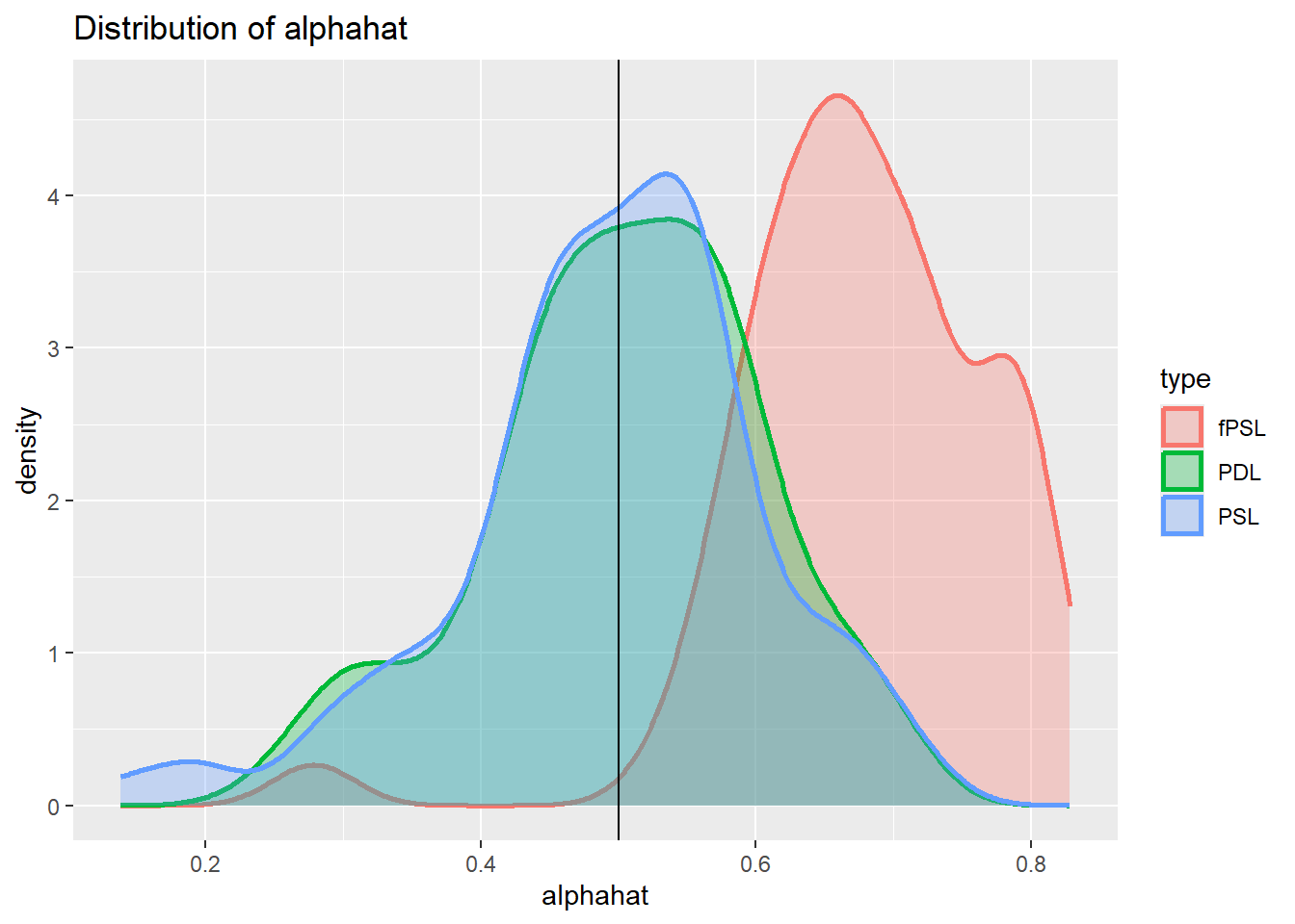
You can see from here that we get a bias in the fPSL estimator but none in the PSL and PDL estimators (the vertical line represents the true coefficient \(\alpha = 0.5\)). This mirrors the results from the Fitzgerald Sice paper, indicating that the PDL offers significant advantages to the fPSL but not to the PSL estimator.
Imperfect confounder overlap 1
From the DGP used in the previous simulation to advantage of the PDL is not apparent. Here we tweak the DGP in one particular way. In the previous dgp it was the same variables in X that were relevant for y and for d. In dgp2 we ensure that the first variable, which is the most important covariate in X for Y, is not relevant for D. At the same time we increase c3 to ensure that approximately the same amount of variation in D can be explained.
dgp2 <- function(n){
    # Simulates Fitzgerald Sice et al
    #  DGP from Section 3.1
    #   d = x * beta_3 + nu
    #   y = delta D + x * beta_1 + epsilon

    eps <- rnorm(n)
    nu <- rnorm(n)

    # Simulates j = 200 variables of X ~ N(0, Sigma)
    J = 200
    mu = rep(0, J)# mean is 0 for all j
    rho <- 0.5  # Define the decay factor FOR CORR MATRIX
    first_row <- rho^(0:(J - 1))
    Sigma <- toeplitz(first_row)   # Generate the covariance matrix using toeplitz
    x <- mvrnorm(n, mu, Sigma)

    # parameters
    c1 <- 0.3
    c3 <- 2.4
    delta <- 0.5
    beta0 <- 1/(seq(1,J,1)^2)
    beta0 <- as.matrix(beta0, J, 1)
    beta1 <- c1 * beta0
    beta3 <- c3 * beta0
    beta3[1] <- 0  # set first coefficient to 0

    # generate d and y
    d <- x %*% beta3 + nu
    y <- delta*d + x %*% beta1 + eps
    return(list(y,d,x))
}

data <- dgp2(1000)
ysim <- unlist(data[[1]])
dsim <- unlist(data[[2]])
xsim <- unlist(data[[3]])

Regy <- summary(lm(ysim~., data.frame(ysim,xsim)))
Regd <- summary(lm(dsim~., data.frame(dsim,xsim)))
paste("R^2 in y equation =", Regy$r.squared)
[1] "R^2 in y equation = 0.437915617484827"paste("R^2 in d equation =", Regd$r.squared)[1] "R^2 in d equation = 0.58711316478842"We can now repeat the simulation
nsim = 100

save_alphahat.dgp2 <- matrix(NA,nrow = nsim, ncol = 3)

for (i in 1:nsim){
  data <- dgp2(100)
  y.sim <- unlist(data[[1]])
  colnames(y.sim) <- "Y"
  d.sim <- unlist(data[[2]])
  colnames(d.sim) <- "D"
  x.sim <- unlist(data[[3]])
  colnames(x.sim) <- paste0("X", 1:ncol(x.sim))
  dx.sim <- cbind(d.sim,x.sim)
  colnames(dx.sim) <- c("D",paste0("X", 1:ncol(x.sim)))

  # fPSL estimator
  pL.reg.fPSL <- fPSL(y.sim,dx.sim)
  save_alphahat.dgp2[i,1] <- pL.reg.fPSL$coefficients["D"]

  # PSL estimator
  pL.reg.PSL <- PSL(y.sim, d.sim, x.sim)
  save_alphahat.dgp2[i,2] <- pL.reg.PSL$coefficients["D"]

  # PDL estimator
  doubleL = rlassoEffect(x = x.sim, y = y.sim, d = d.sim, method = "double selection")
  save_alphahat.dgp2[i,3] <- doubleL$coefficient["D"]
}
Now we can plot the distribution for the two different estimates.
save_alphahat.dgp2 <- as.data.frame(save_alphahat.dgp2) %>%
                  rename(fPSL = V1,
                         PSL = V2,
                         PDL = V3)
#create long dataframe, better for plotting
save_alphahat.dgp2 <- save_alphahat.dgp2 %>% pivot_longer(everything(),names_to = "type", values_to = "alphahat")

plot_den_alphahat.dgp2 <- ggplot(save_alphahat.dgp2, aes(x = alphahat, colour = type, fill = type)) +
  geom_density(alpha = .3, size = 1) +
  geom_vline(aes(xintercept = 0.5)) +
  labs(title = "Distribution of alphahat")
plot_den_alphahat.dgp2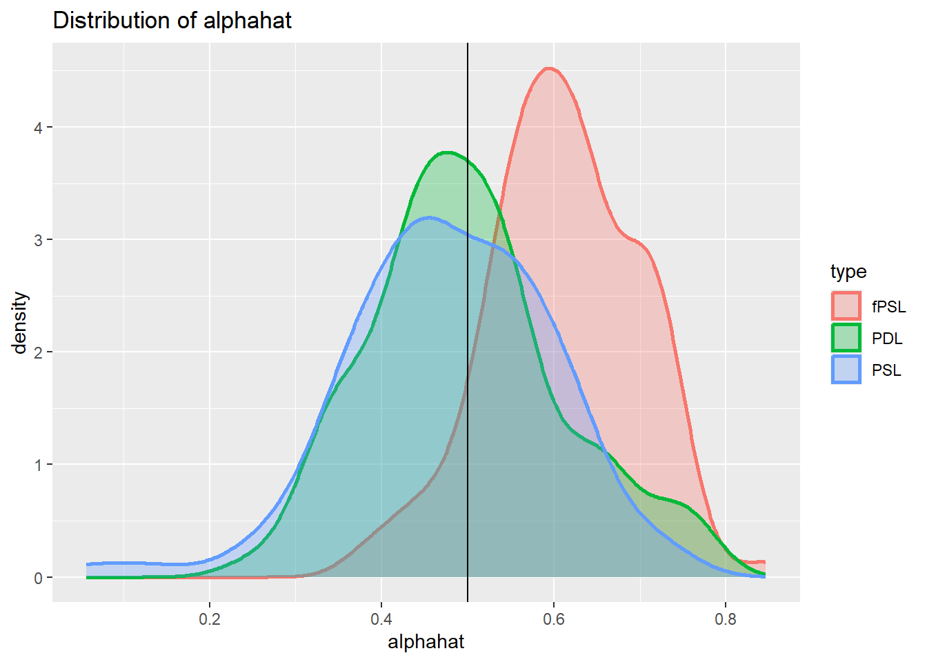
Imperfect confounder overlap 2
The change in DGP we investigate here is that in dgp3 we ensure that the first variable, which is the most important covariate in X for D, is not relevant for Y and therefore unlikely to be picked up by the LASSO for y. However the variable is also correlated to the next variable in X. At the same time we increase c1 to ensure that approximately the same amount of variation in D can be explained.
dgp3 <- function(n){
    # Simulates Fitzgerald Sice et al
    #  DGP from Section 3.1
    #   d = x * beta_3 + nu
    #   y = delta D + x * beta_1 + epsilon

    eps <- rnorm(n)
    nu <- rnorm(n)

    # Simulates j = 200 variables of X ~ N(0, Sigma)
    J = 200
    mu = rep(0, J)# mean is 0 for all j
    rho <- 0.5  # Define the decay factor FOR CORR MATRIX
    first_row <- rho^(0:(J - 1))
    Sigma <- toeplitz(first_row)   # Generate the covariance matrix using toeplitz
    x <- mvrnorm(n, mu, Sigma)

    # parameters
    c1 <- 0.6
    c3 <- 0.8
    delta <- 0.5
    beta0 <- 1/(seq(1,J,1)^2)
    beta0 <- as.matrix(beta0, J, 1)
    beta1 <- c1 * beta0
    beta3 <- c3 * beta0
    beta1[1] <- 0  # set first coefficient to 0

    # generate d and y
    d <- x %*% beta3 + nu
    y <- delta*d + x %*% beta1 + eps
    return(list(y,d,x))
}

data <- dgp3(1000)
ysim <- unlist(data[[1]])
dsim <- unlist(data[[2]])
xsim <- unlist(data[[3]])

Regy <- summary(lm(ysim~., data.frame(ysim,xsim)))
Regd <- summary(lm(dsim~., data.frame(dsim,xsim)))
paste("R^2 in y equation =", Regy$r.squared)
[1] "R^2 in y equation = 0.41187670865023"paste("R^2 in d equation =", Regd$r.squared)[1] "R^2 in d equation = 0.58323287658988"We can now repeat the simulation
nsim = 100

save_alphahat.dgp3 <- matrix(NA,nrow = nsim, ncol = 3)

for (i in 1:nsim){
  data <- dgp3(100)
  y.sim <- unlist(data[[1]])
  colnames(y.sim) <- "Y"
  d.sim <- unlist(data[[2]])
  colnames(d.sim) <- "D"
  x.sim <- unlist(data[[3]])
  colnames(x.sim) <- paste0("X", 1:ncol(x.sim))
  dx.sim <- cbind(d.sim,x.sim)
  colnames(dx.sim) <- c("D",paste0("X", 1:ncol(x.sim)))

  # fPSL estimator
  pL.reg.fPSL <- fPSL(y.sim,dx.sim)
  save_alphahat.dgp3[i,1] <- pL.reg.fPSL$coefficients["D"]

  # PSL estimator
  pL.reg.PSL <- PSL(y.sim, d.sim, x.sim)
  save_alphahat.dgp3[i,2] <- pL.reg.PSL$coefficients["D"]

  # PDL estimator
  doubleL = rlassoEffect(x = x.sim, y = y.sim, d = d.sim, method = "double selection")
  save_alphahat.dgp3[i,3] <- doubleL$coefficient["D"]
}
Now we can plot the distribution for the two different estimates.
save_alphahat.dgp3 <- as.data.frame(save_alphahat.dgp3) %>%
                  rename(fPSL = V1,
                         PSL = V2,
                         PDL = V3)
#create long dataframe, better for plotting
save_alphahat.dgp3 <- save_alphahat.dgp3 %>% pivot_longer(everything(),names_to = "type", values_to = "alphahat")

plot_den_alphahat.dgp3 <- ggplot(save_alphahat.dgp3, aes(x = alphahat, colour = type, fill = type)) +
  geom_density(alpha = .3, size = 1) +
  geom_vline(aes(xintercept = 0.5)) +
  labs(title = "Distribution of alphahat")
plot_den_alphahat.dgp3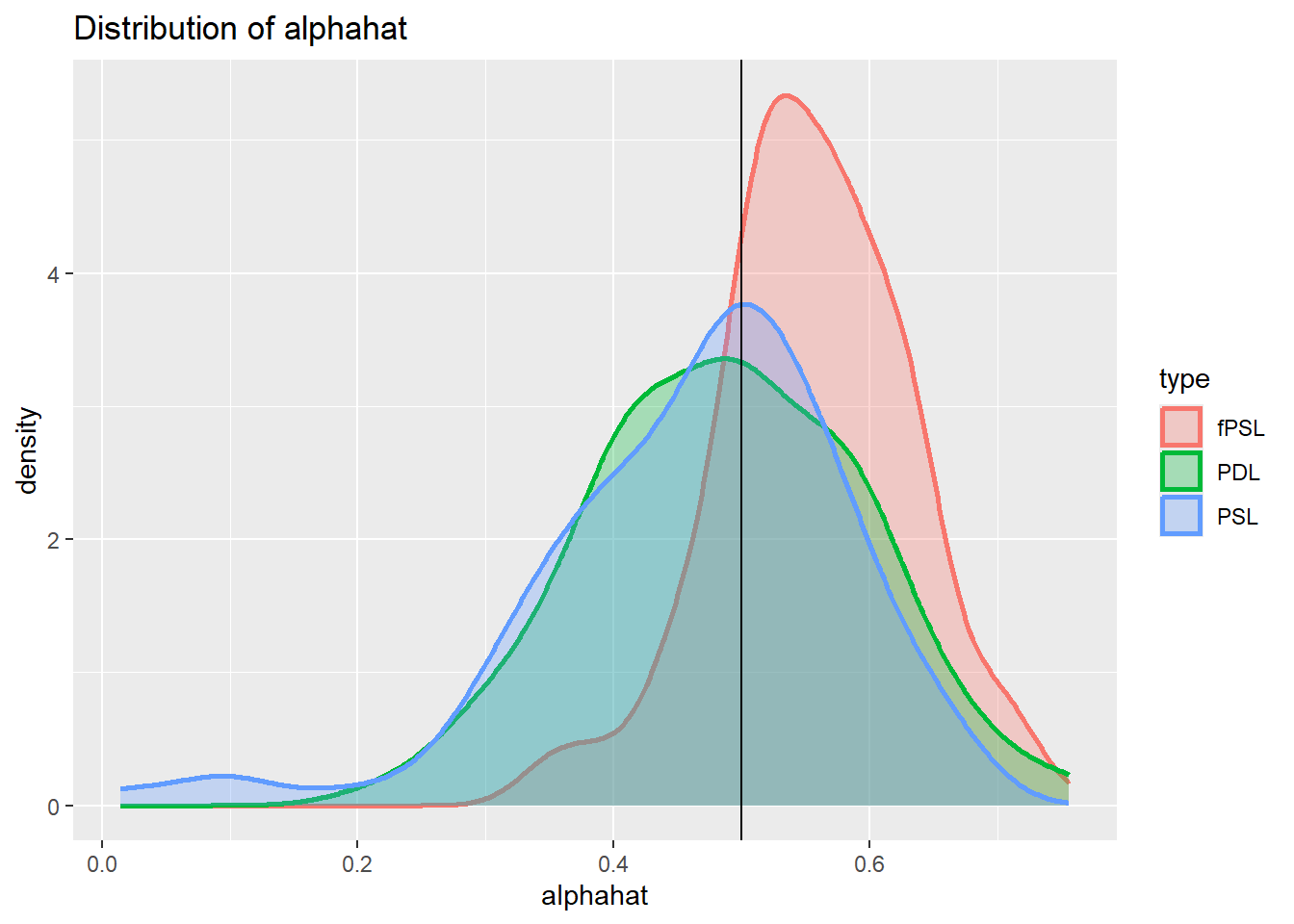
Inclusion of instruments
This setup illustrates when there are variables in X that are not part of the y equation but do explain variation in the treatment variable D. Such variables are of course instruments and they would allow an instrumental variable estimation approach to recover the causal affect of D on y.
In the simulation we obtain such a setup as follows. The simulation sets up a set of 200 variables in the matrix X. Only the first few are relevant for explaining y as the base vector beta0 is setup as beta0 <- 1/(seq(1,J,1)^2) implying a sequence of values \(1, 1/4, 1/9, 1/16, etc.\) The result being that only the first few variables explain variation in y. In dgp1 it is the same first few elements in X that explain variation in the treatment variable D. In dgp2 and dgp3 they were basically the same again, just that we switched some off either for the y or D equation, but fundamentally tehy were still the same.
In this DGP we turn around the order of variables that explain y and D. y remains explained by the first few variables in X while D is explained by the last few variables in X. We achieve this by reversing the order of beta0 when setting beta3. This will ensure that the covariates that explain variationin y are not the same as the elements in X that explain variation in D. As now the variables that are explain in D can be excluded from the y equation, these are essentially instruments. Note that they are also virtually uncorrelated to the other elements in X that are included in the y equation.
dgp3 <- function(n){
    # Simulates Fitzgerald Sice et al
    #  DGP from Section 3.1
    #   d = x * beta_3 + nu
    #   y = delta D + x * beta_1 + epsilon

    eps <- rnorm(n)
    nu <- rnorm(n)

    # Simulates j = 200 variables of X ~ N(0, Sigma)
    J = 200
    mu = rep(0, J)# mean is 0 for all j
    rho <- 0.5  # Define the decay factor FOR CORR MATRIX
    first_row <- rho^(0:(J - 1))
    Sigma <- toeplitz(first_row)   # Generate the covariance matrix using toeplitz
    x <- mvrnorm(n, mu, Sigma)

    # parameters
    c1 <- 0.3
    c3 <- 0.8
    delta <- 0.5
    beta0 <- 1/(seq(1,J,1)^2)
    beta0 <- as.matrix(beta0, J, 1)
    beta1 <- c1 * beta0
    beta3 <- c3 * as.matrix(rev(beta0), J, 1) # reverse beta0


    # generate d and y
    d <- x %*% beta3 + nu
    y <- delta*d + x %*% beta1 + eps
    return(list(y,d,x))
}

data <- dgp2(1000)
ysim <- unlist(data[[1]])
dsim <- unlist(data[[2]])
xsim <- unlist(data[[3]])

Regy <- summary(lm(ysim~., data.frame(ysim,xsim)))
Regd <- summary(lm(dsim~., data.frame(dsim,xsim)))
paste("R^2 in y equation =", Regy$r.squared)
[1] "R^2 in y equation = 0.478032593726361"paste("R^2 in d equation =", Regd$r.squared)[1] "R^2 in d equation = 0.599804740636386"We can now repeat the simulation
nsim = 100

save_alphahat.dgp3 <- matrix(NA,nrow = nsim, ncol = 3)

for (i in 1:nsim){
  data <- dgp3(100)
  y.sim <- unlist(data[[1]])
  colnames(y.sim) <- "Y"
  d.sim <- unlist(data[[2]])
  colnames(d.sim) <- "D"
  x.sim <- unlist(data[[3]])
  colnames(x.sim) <- paste0("X", 1:200)
  dx.sim <- cbind(d.sim,x.sim)
  colnames(dx.sim) <- c("D",paste0("X", 1:200))

  # fPSL estimator
  pL.reg.fPSL <- fPSL(y.sim,dx.sim)
  save_alphahat.dgp3[i,1] <- pL.reg.fPSL$coefficients["D"]

  # PSL estimator
  pL.reg.PSL <- PSL(y.sim, d.sim, x.sim)
  save_alphahat.dgp3[i,2] <- pL.reg.PSL$coefficients["D"]

  # PDL estimator
  doubleL = rlassoEffect(x = x.sim, y = y.sim, d = d.sim, method = "double selection")
  save_alphahat.dgp3[i,3] <- doubleL$coefficient["D"]
}
Now we can plot the distribution for the three different estimates.
save_alphahat.dgp3 <- as.data.frame(save_alphahat.dgp3) %>%
                  rename(fPSL = V1,
                         PSL = V2,
                         PDL = V3)
#create long dataframe, better for plotting
save_alphahat.dgp3 <- save_alphahat.dgp3 %>% pivot_longer(everything(),names_to = "type", values_to = "alphahat")

plot_den_alphahat.dgp3 <- ggplot(save_alphahat.dgp3, aes(x = alphahat, colour = type, fill = type)) +
  geom_density(alpha = .3, size = 1) +
  geom_vline(aes(xintercept = 0.5)) +
  labs(title = "Distribution of alphahat")
plot_den_alphahat.dgp3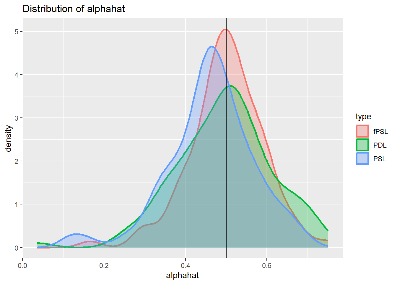
In this case, the Double Lasso will ensure that the instruments are included in the post regression, but their inclusion does not harm the PDL.
Unobserved confounders
Now we will simulate a situation in which there is an unobserved confounder, i.e. a variable that explains variation, both in D and y but cannot be observed and therefore cannot be included in any empirical regresison models.
dgp4 <- function(n){
    # Simulates Fitzgerald Sice et al
    #  DGP from Section 3.1
    #   d = x * beta_3 + nu
    #   y = delta D + x * beta_1 + epsilon

    eps <- rnorm(n)
    nu <- rnorm(n)
    u <- rnorm(n)  # unobserved confounder

    # Simulates j = 200 variables of X ~ N(0, Sigma)
    J = 200
    mu = rep(0, J)# mean is 0 for all j
    rho <- 0.5  # Define the decay factor FOR CORR MATRIX
    first_row <- rho^(0:(J - 1))
    Sigma <- toeplitz(first_row)   # Generate the covariance matrix using toeplitz
    x <- mvrnorm(n, mu, Sigma)

    # parameters
    c1 <- 0.3
    c3 <- 0.8
    delta <- 0.5
    beta0 <- 1/(seq(1,J,1)^2)
    beta0 <- as.matrix(beta0, J, 1)
    beta1 <- c1 * beta0
    beta3 <- c3 * beta0

    gamma1 = 0.5
    gamma3 = 0.4

    # generate d and y
    d <- x %*% beta3 + gamma3*u + nu
    y <- delta*d + x %*% beta1 + gamma1*u + eps
    return(list(y,d,x))
}

data <- dgp4(1000)
ysim <- unlist(data[[1]])
dsim <- unlist(data[[2]])
xsim <- unlist(data[[3]])

Regy <- summary(lm(ysim~., data.frame(ysim,xsim)))
Regd <- summary(lm(dsim~., data.frame(dsim,xsim)))
paste("R^2 in y equation =", Regy$r.squared)
[1] "R^2 in y equation = 0.423316158782026"paste("R^2 in d equation =", Regd$r.squared)[1] "R^2 in d equation = 0.555845894021418"We can now repeat the simulation
nsim = 100

save_alphahat.dgp4 <- matrix(NA,nrow = nsim, ncol = 3)

for (i in 1:nsim){
  data <- dgp4(100)
  y.sim <- unlist(data[[1]])
  colnames(y.sim) <- "Y"
  d.sim <- unlist(data[[2]])
  colnames(d.sim) <- "D"
  x.sim <- unlist(data[[3]])
  colnames(x.sim) <- paste0("X", 1:200)
  dx.sim <- cbind(d.sim,x.sim)
  colnames(dx.sim) <- c("D",paste0("X", 1:200))

  # fPSL estimator
  pL.reg.fPSL <- fPSL(y.sim,dx.sim)
  save_alphahat.dgp4[i,1] <- pL.reg.fPSL$coefficients["D"]

  # PSL estimator
  pL.reg.PSL <- PSL(y.sim, d.sim, x.sim)
  save_alphahat.dgp4[i,2] <- pL.reg.PSL$coefficients["D"]

  # PDL estimator
  doubleL = rlassoEffect(x = x.sim, y = y.sim, d = d.sim, method = "double selection")
  save_alphahat.dgp4[i,3] <- doubleL$coefficient["D"]
}
Now we can plot the distribution for the three different estimates.
save_alphahat.dgp4 <- as.data.frame(save_alphahat.dgp4) %>%
                  rename(fPSL = V1,
                         PSL = V2,
                         PDL = V3)
#create long dataframe, better for plotting
save_alphahat.dgp4 <- save_alphahat.dgp4 %>% pivot_longer(everything(),names_to = "type", values_to = "alphahat")

plot_den_alphahat.dgp4 <- ggplot(save_alphahat.dgp4, aes(x = alphahat, colour = type, fill = type)) +
  geom_density(alpha = .3, size = 1) +
  geom_vline(aes(xintercept = 0.5)) +
  labs(title = "Distribution of alphahat")
plot_den_alphahat.dgp4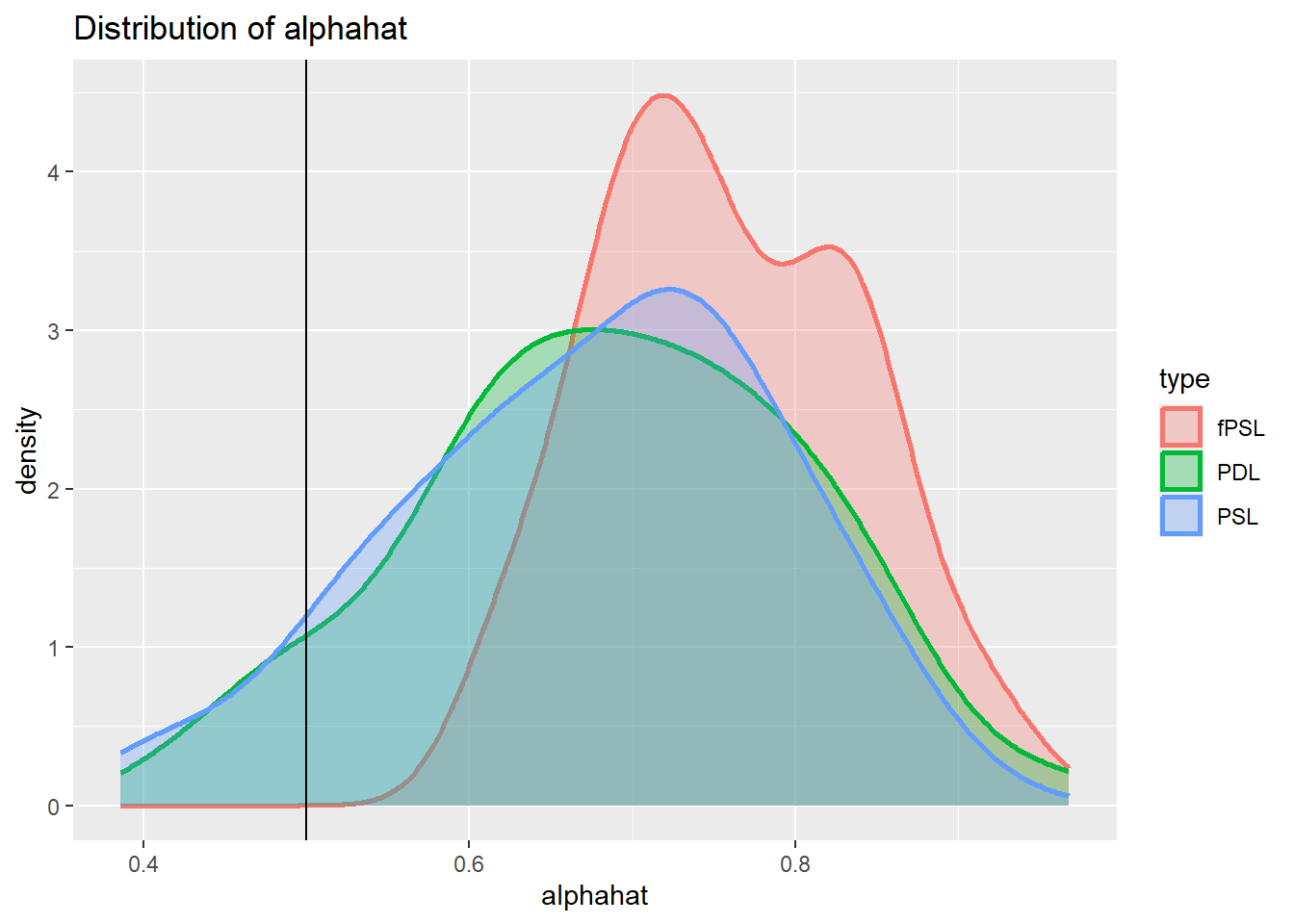
It is apparent from tehse histograms that all estimators show a clear bias under these circumstance. But this is not really a surprise, the methods proposed here are designed to improve causal inference when selection driven by observable variables.
If there are unobserved confounders different research designs are called for.
Reading
- Belloni, A., V. Chernozhukov and C. Hansen (2014), Inference on Treatment Effects After Selection Among High-dimensional Controls, The Review of Economic Studies, 81, 2369-2429.
- Fitzgerald Sice, Jack and Lattimore, Finnian and Robinson, Tim and Zhu, Anna, Practical Insights Into Applying Double LASSO (May 18, 2023). Available at SSRN: https://ssrn.com/abstract=4452778 or http://dx.doi.org/10.2139/ssrn.4452778