%load_ext pretty_jupyter
Introduction
This walk-through is part of the ECLR page.
In this walkthrough you will learn to
- use SQL to access database
- select rows and variables from a single database table
- join data from multiple tables in a database
- aggregate data
- calculate new variables
You have been studying Python such that you can do simple or very complex data analysis. Why would you need to know SQL (which stands for Structured Query Language)? These days all large (and some small) businesses keep enourmous amounts of data (think every interaction you as a customer may have with the Amazon webpage). These data are saved in what are called databases. Databases are really collections of spreadsheets (with observations in rows and variables in columns). Often the data is organised such that different spreadsheets can potentially be linked as they have common keys. Such databases are called relational databases.
There may be a lot of interesting analysis you could do with some of the data in such a database. However, these databases are often so big that you will have to first extract some suitable subset of the data (perhaps already aggregated to a certain level) such that the dataset's structure and size is suitable for analysis in Python.
The language used to access and extract data is SQL and it stands at the beginning of many data projects. The result of SQL work is typically not the analysis of your data itself, but rather the particular data on which you then perform the analysis.
Database setup
Unsurprisingly databases come in different formats. However, the good thing is that communicating with these always happens with variants of the SQL language. For certain applications and database formats you can access databases directly from Python. This is what we will cover here, we assume that a database is stored locally and then we use Python to communicate with that database.
In commercial organisations, where datbases are accessed by many people independently and simultaneously, this access needs to be controlled by a database server. But here we will abstract from such difficulties. When you work in a particular organisation you will be introduced to any such specifics.
We use an example database that has been created for teaching purposes called northwind.db. This is built as a SQLlite type database which can just be saved locally on your computer without the need for a server. As such in can then be directly accessed from, say, Python.
Go to JP White's github page and download the northwind.db database file and save it into your data directory (or directory you are working from).
Next we install libraries we will be using in this workthrough. Importantly, one of them is the sqlite3 library which will allow us to communicate with the SQLite formatted database northwind.db.
import pandas as pd
import numpy as np
import sqlite3
from lets_plot import *
import statsmodels.api as sm
# Lets_plot requires a setup
LetsPlot.setup_html(no_js=True)
Before we continue we shall test whether we can connect to the database. Run the following command and you should get the following output.
con = sqlite3.connect("../data/northwind.db")
pd.read_sql_query("SELECT COUNT(*) AS n FROM Orders;", con)
| n | |
|---|---|
| 0 | 16282 |
Without talking about the detail of this query, this output tells you that there are more than 16K rows of data in the Orders spreadsheet.
The only coding aspect we need to take from this is how the SQL code to communicate with the database is delivered. It is delivered as a text command inside the pd.read_sql_query function. The second input into the function is con which was defined above. con is the connection to the database and we will need it whenever we communicate with the database.
pd.read_sql_query("SQL code finished with a ;", con)
Exploring the database
A database will often have many different tables. Think an EXCEL file with multiple sheets. When working with a database it is important to understand the structure of the database, meaning, which tables does it contain and which variables are in each table. Understanding which variables are contained in each table is important so that we can link data from different tables.
You can see a structure of the database on JP White's github page for the northwind database.
Identify tables
We use the following command to get the names of the tables contained in the Nortwind database.
pd.read_sql_query("SELECT name FROM sqlite_master WHERE type='table';", con)
| name | |
|---|---|
| 0 | Categories |
| 1 | sqlite_sequence |
| 2 | CustomerCustomerDemo |
| 3 | CustomerDemographics |
| 4 | Customers |
| 5 | Employees |
| 6 | EmployeeTerritories |
| 7 | Order Details |
| 8 | Orders |
| 9 | Products |
| 10 | Regions |
| 11 | Shippers |
| 12 | Suppliers |
| 13 | Territories |
Finding code
Websearch
As we are at the beginning of our SQL learning journey you cannot be expected to know how to get a list of the tables from the database. You could use your favourite search engine and search for something like "How to use SQL to get all table names in a database sqlite". In my case this led me to the following website that provides quite clear but wordy instruction on how to do that.
This will give the SQL command that needs to be inserted into the pd.read_sql_query function.
AI
You could also ask your favourite AI engine. But you will have to give the AI enough information. For instance you could ask the following: "I am working in Python and am accessing a SQLite database called "northwind.db". How can I get a list of all tables in the database?"
This database has 13 tables. It represents the database for a small company with customers, inventory, purchasing, suppliers, employees etc.
Accessing data from a table
Let's say we want to access data from the Suppliers table. It will be important to know what variables are included in this table.
pd.read_sql_query("PRAGMA table_info(Suppliers);", con)
| cid | name | type | notnull | dflt_value | pk | |
|---|---|---|---|---|---|---|
| 0 | 0 | SupplierID | INTEGER | 1 | None | 1 |
| 1 | 1 | CompanyName | TEXT | 1 | None | 0 |
| 2 | 2 | ContactName | TEXT | 0 | None | 0 |
| 3 | 3 | ContactTitle | TEXT | 0 | None | 0 |
| 4 | 4 | Address | TEXT | 0 | None | 0 |
| 5 | 5 | City | TEXT | 0 | None | 0 |
| 6 | 6 | Region | TEXT | 0 | None | 0 |
| 7 | 7 | PostalCode | TEXT | 0 | None | 0 |
| 8 | 8 | Country | TEXT | 0 | None | 0 |
| 9 | 9 | Phone | TEXT | 0 | None | 0 |
| 10 | 10 | Fax | TEXT | 0 | None | 0 |
| 11 | 11 | HomePage | TEXT | 0 | None | 0 |
What is PRAGMA
SQLite specific solution
The above code using the PRAGMA command is a solution to the particular problem at hand using a SQLite specific command the PRAGMA command. It makes certain things much easier than using SQL language that is universal across different database formats. But if your database is not in the SQLite format, then this will not be available.
A generic SQL solution
If you want to get a list of variables in a table in a way that should be applicable across different database formats you do the following:
cursor = con.cursor()
cursor.execute("SELECT * FROM Suppliers LIMIT 0;")
columns = [desc[0] for desc in cursor.description]
print(columns)
['SupplierID', 'CompanyName', 'ContactName', 'ContactTitle', 'Address', 'City', 'Region', 'PostalCode', 'Country', 'Phone', 'Fax', 'HomePage']
As you can see this merely prints a list variables and we will not go through the details of this command here.
The reality is that you may be able to find easier solutions specific to your particular database format.
Now we may wish to look at the Suppliers database and find all the suppliers that are from the UK. Let's see how this works and then we will disect the command (which is again delivered via the pd.read_sql_query function).
pd.read_sql_query("SELECT CompanyName, City FROM Suppliers WHERE Country = 'UK' \
ORDER BY CompanyName;", con)
| CompanyName | City | |
|---|---|---|
| 0 | Exotic Liquids | London |
| 1 | Specialty Biscuits, Ltd. | Manchester |
First, note that the line break is indicated by "\". It is important that there is no space after the "\".
If you wish to save the results of this query into a spreadsheet you can do this as follows. First save the query in a DataFrame and then save that using the to_csv method.
uk_suppliers = pd.read_sql_query("SELECT CompanyName, City FROM Suppliers WHERE Country = 'UK' \
ORDER BY CompanyName;", con)
uk_suppliers.to_csv('uk_suppliers.csv', index=False)
When looking at the result it becomes obvious what the above SQL command did.
# selects variables CompanyName and City from the Suppliers table
SELECT CompanyName, City FROM Suppliers
# but only the rows where country is equal to UK
WHERE Country = 'UK'
# Then order the result by CompanyName
ORDER BY CompanyName;
Practice Exercise
Task
Using the Products table, find out of which products the company has more than 100 units in stock (UnitsInStock > 100). Create a table with these products and include the following variables into the table: ProductName, QuantityPerUnit, MinOrderAmount, UnitsInStock. But check whether all these variables actually exist in the Products table.
Solution Strategy
First check which of the above four variables actually do exist. Adjust the earlier PRAGMA command to achieve this.
Then, you should adjust the above SELECT ... FROM ... WHERE command to the question at hand.
Solution
First check which variables are available in Products.
pd.read_sql_query("PRAGMA table_info(Products);", con)
| cid | name | type | notnull | dflt_value | pk | |
|---|---|---|---|---|---|---|
| 0 | 0 | ProductID | INTEGER | 1 | None | 1 |
| 1 | 1 | ProductName | TEXT | 1 | None | 0 |
| 2 | 2 | SupplierID | INTEGER | 0 | None | 0 |
| 3 | 3 | CategoryID | INTEGER | 0 | None | 0 |
| 4 | 4 | QuantityPerUnit | TEXT | 0 | None | 0 |
| 5 | 5 | UnitPrice | NUMERIC | 0 | 0 | 0 |
| 6 | 6 | UnitsInStock | INTEGER | 0 | 0 | 0 |
| 7 | 7 | UnitsOnOrder | INTEGER | 0 | 0 | 0 |
| 8 | 8 | ReorderLevel | INTEGER | 0 | 0 | 0 |
| 9 | 9 | Discontinued | TEXT | 1 | '0' | 0 |
Now we know that only ProductName, QuantityPerUnit and UnitsInStock do exist. The following command selects these three variables, using the condition WHERE UnitsInStock > 100.
pd.read_sql_query("SELECT ProductName, QuantityPerUnit, UnitsInStock FROM Products \
WHERE UnitsInStock > 100 \
ORDER BY UnitsInStock;", con)
| ProductName | QuantityPerUnit | UnitsInStock | |
|---|---|---|---|
| 0 | Röd Kaviar | 24 - 150 g jars | 101 |
| 1 | Gustaf's Knäckebröd | 24 - 500 g pkgs. | 104 |
| 2 | Sasquatch Ale | 24 - 12 oz bottles | 111 |
| 3 | Geitost | 500 g | 112 |
| 4 | Inlagd Sill | 24 - 250 g jars | 112 |
| 5 | Sirop d'érable | 24 - 500 ml bottles | 113 |
| 6 | Pâté chinois | 24 boxes x 2 pies | 115 |
| 7 | Grandma's Boysenberry Spread | 12 - 8 oz jars | 120 |
| 8 | Boston Crab Meat | 24 - 4 oz tins | 123 |
| 9 | Rhönbräu Klosterbier | 24 - 0.5 l bottles | 125 |
Grouping and Aggregating Data
Often you will find that a database contains information on individual customers or individual transactions. The amount of data can be very large and for an analysis you may not be interested in the individual observations but rather in aggregated information. If so, then it may not be necessary to download the individual observations but it would be possible to aggregate information, for instance to a daily transaction summaries, which can then be downloaded for analysis.
The first task we will undertake is to summarise the number of orders (from the Orders table) that go to different countries.
Understand the structure of Orders
Question
Before proceeding with this you will want to check out what variables are included in the Orders table and in particular what the variable is called that contains the country information. Attempt to apply the previously introduced PRAGMA table_info(NAME_OF_TABLE); command (recall that this is convenient but specific to SQLite databases) to find the names of the variables.
Solution
pd.read_sql_query("PRAGMA table_info(Orders);", con)
| cid | name | type | notnull | dflt_value | pk | |
|---|---|---|---|---|---|---|
| 0 | 0 | OrderID | INTEGER | 1 | None | 1 |
| 1 | 1 | CustomerID | TEXT | 0 | None | 0 |
| 2 | 2 | EmployeeID | INTEGER | 0 | None | 0 |
| 3 | 3 | OrderDate | DATETIME | 0 | None | 0 |
| 4 | 4 | RequiredDate | DATETIME | 0 | None | 0 |
| 5 | 5 | ShippedDate | DATETIME | 0 | None | 0 |
| 6 | 6 | ShipVia | INTEGER | 0 | None | 0 |
| 7 | 7 | Freight | NUMERIC | 0 | 0 | 0 |
| 8 | 8 | ShipName | TEXT | 0 | None | 0 |
| 9 | 9 | ShipAddress | TEXT | 0 | None | 0 |
| 10 | 10 | ShipCity | TEXT | 0 | None | 0 |
| 11 | 11 | ShipRegion | TEXT | 0 | None | 0 |
| 12 | 12 | ShipPostalCode | TEXT | 0 | None | 0 |
| 13 | 13 | ShipCountry | TEXT | 0 | None | 0 |
From here you learn that the variable we are interested in is called ShipCountry
Now that we know the variable name of the country variable we can look at how many orders there are. Let's, for a moment, imagine you had a dataframe in Python called Orders which had a variable called ShipCountry. How would achieve this in Python?
Orders.groupby('ShipCountry').size()
So there were two elements, we needed to group the data by the ShipCountry variable and then count, which here was achieved by using the size() method which counts the number of observations in each group. Similar tasks have to be achieved when using a SQL query to the database.
Here is the command used:
pd.read_sql_query("SELECT ShipCountry, COUNT(*) AS n_orders FROM Orders GROUP BY ShipCountry ORDER BY n_orders DESC;", con)
| ShipCountry | n_orders | |
|---|---|---|
| 0 | USA | 2328 |
| 1 | Germany | 2193 |
| 2 | France | 1778 |
| 3 | Brazil | 1683 |
| 4 | UK | 1280 |
| 5 | Mexico | 899 |
| 6 | Venezuela | 707 |
| 7 | Spain | 691 |
| 8 | Canada | 547 |
| 9 | Italy | 538 |
| 10 | Argentina | 535 |
| 11 | Sweden | 391 |
| 12 | Austria | 380 |
| 13 | Finland | 369 |
| 14 | Switzerland | 367 |
| 15 | Portugal | 357 |
| 16 | Denmark | 352 |
| 17 | Belgium | 338 |
| 18 | Poland | 213 |
| 19 | Ireland | 172 |
| 20 | Norway | 164 |
What does this command do?
Question
We want to disect this command as it helps us understand how SQL works. Can you identify the equivalents to groupby and size()?
Solution
Here is a detailed breakdown:
Start by retrieving the ShipCountry column from Orders and COUNT the rows
SELECT ShipCountry, COUNT(*) AS n_orders FROM Orders
You can try and run this command alone and see what happens. Basically you will have selected one variable and then you counted all the rows in the table. At this stage you have counted but not grouped. This is achieved by the following:
GROUP BY ShipCountry
and finally you can order the result by n_orders:
ORDER BY n_orders DESC;
As you can see from the above examples, the outcome of working with databases is usually a table. Usually we use SQL to assemble data which are then presented in a table for further analysis in Python. So working with databases is typically a preliminary step to some data analysis. And the reason for this, in real life, is that often the amount of data contained in databases exceeds what we actually need and hence we reduce the size of the dataset before we start analysing. This reduction will often be in terms of just selecting subsets of data or by aggregating data, both of which we practised above.
Joining data
Apart from filtering and aggregating data there is a third very common operation you will have to do when working with databases, namely joining databases. In Python you may have merged dataframes and basically joining (in SQL) and merging (in Python) are the same conceptual tasks.
Let's join information from the Orders, Order Details and the Customers tables in order to find which customers are most valuable to the Northwind company. Above we already looked at the variables in the Orders table. Let us now look at the variables in Order Details as the information in Orders didn't actually contain any details, like product values. These can be calculated from the data in Order Details as that table contains UnitPrice, Quantity and Discount on the basis of which we can calculate an order value.
pd.read_sql_query("PRAGMA table_info('Order Details');", con)
| cid | name | type | notnull | dflt_value | pk | |
|---|---|---|---|---|---|---|
| 0 | 0 | OrderID | INTEGER | 1 | None | 1 |
| 1 | 1 | ProductID | INTEGER | 1 | None | 2 |
| 2 | 2 | UnitPrice | NUMERIC | 1 | 0 | 0 |
| 3 | 3 | Quantity | INTEGER | 1 | 1 | 0 |
| 4 | 4 | Discount | REAL | 1 | 0 | 0 |
The following image demonstrates how these three tables can be linked. The variables CustomerID and OrderID, both of which occur in multiple tables allow us to link the data.
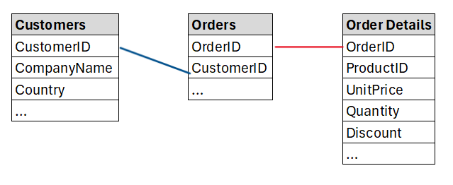
The initial plan is to create a new table which contains CustomerID, CustomerName, Country, Order ID, UnitPrice and Quantity. We expect to create a table with as many rows as the the Order table.
Let's begin by creating a table that adds the customer name and country to the information in Orders.
pd.read_sql_query("SELECT o.OrderID, c.CompanyName ,c.Country FROM Orders o\
JOIN Customers c ON o.CustomerID = c.CustomerID;", con)
| OrderID | CompanyName | Country | |
|---|---|---|---|
| 0 | 10248 | Vins et alcools Chevalier | France |
| 1 | 10249 | Toms Spezialitäten | Germany |
| 2 | 10250 | Hanari Carnes | Brazil |
| 3 | 10251 | Victuailles en stock | France |
| 4 | 10252 | Suprêmes délices | Belgium |
| ... | ... | ... | ... |
| 16277 | 26525 | White Clover Markets | USA |
| 16278 | 26526 | Wolski Zajazd | Poland |
| 16279 | 26527 | Gourmet Lanchonetes | Brazil |
| 16280 | 26528 | Blondesddsl père et fils | France |
| 16281 | 26529 | Du monde entier | France |
16282 rows × 3 columns
What does this command do?
Question
We want to understand how to join/merge datasets in SQL. What are the important elements of this command?
Solution
Here is a detailed breakdown:
We start by selecting columns, in particular the OrderID info from the Orders table and the CompanyName and Country columns from the Customers table.
SELECT o.OrderID, c.CompanyName ,c.Country FROM Orders o
The variable from the Orders table was prefixed with o. and the ones from the Customers table with c. The prefix o. was defined in the FROM Orders o part where we basically gave the Orders table the o. name. The next part will tell SQL where the c. variables are coming from:
JOIN Customers c ON o.CustomerID = c.CustomerID
Here we specify that the the c. variables are being joined in from the Customers table. The crucial piece of information here follows the ON command. Here we say which variables from the Orders and Customers tables should be used to link the data. We know that this should be the CustomerID variable which exists in both tables (o.CustomerID = c.CustomerID).
Here that linking variable has the same name in both tables but they could have different names and you could still link them.Don't forget that a SQL command always concludes with a ;.
As a result we got a table we get a table with 16,282 orders.
Challenge
Task
Amend the above joining to also join in the UnitPrice and Quantity from the Order Details table?
Search Strategy
There are three ways you could work this out.
- Trial and Error. if you have a hunch of how it may work then just give it a go. You cannot break the computer!
- Use a search engine. For instance you could enter a search term like "SQL joining data from three tables SQLite". This then pointed me to a Stackoverflow page which basically had the right solution.
- Use a LLM to find the solution. You need to describe to the LLM what your problem is. In particular you will want to give the LLM enough information to fully describe the complexity of your problem. Here is a chat with ChatGPT in which you can see how to ask.
Solution
Here is the solution.
pd.read_sql_query("SELECT o.OrderID, c.CompanyName ,c.Country, od.UnitPrice, od.Quantity \
FROM Orders o\
JOIN Customers c ON o.CustomerID = c.CustomerID\
JOIN 'Order Details' od ON o.OrderID = od.OrderID;", con)
| OrderID | CompanyName | Country | UnitPrice | Quantity | |
|---|---|---|---|---|---|
| 0 | 10248 | Vins et alcools Chevalier | France | 14.00 | 12 |
| 1 | 10248 | Vins et alcools Chevalier | France | 9.80 | 10 |
| 2 | 10248 | Vins et alcools Chevalier | France | 34.80 | 5 |
| 3 | 10249 | Toms Spezialitäten | Germany | 18.60 | 9 |
| 4 | 10249 | Toms Spezialitäten | Germany | 42.40 | 40 |
| ... | ... | ... | ... | ... | ... |
| 609278 | 26529 | Du monde entier | France | 31.00 | 26 |
| 609279 | 26529 | Du monde entier | France | 12.00 | 18 |
| 609280 | 26529 | Du monde entier | France | 31.23 | 3 |
| 609281 | 26529 | Du monde entier | France | 43.90 | 24 |
| 609282 | 26529 | Du monde entier | France | 39.00 | 26 |
609283 rows × 5 columns
As you can see, joining in data from a third file was not a problem as we merely had to add another JOINing instruction.
The result is a table with 609,238 rows of data. We now have more rows as one order may have orders for multiple products. For instance the forst order 10248 now has three rows as three different products were included in that order. Each row now represents an order for a particular product.
Calculating a new variable
So far you have learned how to select variables and rows from databases, how to aggregate and how to join data. We continue the previous example in which we joined the data from the Orders, Customers and Order Details tables. One of the pieces of information we did get was the UnitPrice and Quantity variables. We can use that to also calculate the OrderValue which we can then use to find the customers who order most from Northwind.
After calculating the OrderValue in each row we can then aggregate by CustomerID to get that information.
To achieve this, you could either save the table we retrieved above and do the calculation in Python, or you can do the calculation as you retrieve the information. Here, as this is a walkthrough to get exposed to SQL, we will do the latter.
pd.read_sql_query("SELECT c.CompanyName ,c.Country, od.UnitPrice * od.Quantity AS OrderValue \
FROM Orders o\
JOIN Customers c ON o.CustomerID = c.CustomerID\
JOIN 'Order Details' od ON o.OrderID = od.OrderID;", con)
| CompanyName | Country | OrderValue | |
|---|---|---|---|
| 0 | Vins et alcools Chevalier | France | 168.00 |
| 1 | Vins et alcools Chevalier | France | 98.00 |
| 2 | Vins et alcools Chevalier | France | 174.00 |
| 3 | Toms Spezialitäten | Germany | 167.40 |
| 4 | Toms Spezialitäten | Germany | 1696.00 |
| ... | ... | ... | ... |
| 609278 | Du monde entier | France | 806.00 |
| 609279 | Du monde entier | France | 216.00 |
| 609280 | Du monde entier | France | 93.69 |
| 609281 | Du monde entier | France | 1053.60 |
| 609282 | Du monde entier | France | 1014.00 |
609283 rows × 3 columns
Why 100.80000000000001 and not 100.8?
Question
If you look at the 9th row (indexed 8) and the OrderValue you will find the result 16.8*6 = 100.80000000000001. Why is that?
- There is no problem, that is the correct result.
- This is a bug of my computer
- Some numbers cannot be precisely represented as binary numbers (which is what computers do) and when they are used tiny errors like the above can result.
- The calculation was done by a LLM and it just gets things wrong.
Solution
Some numbers cannot be precisely represented as binary numbers (which is what computers do) and when they are used tiny errors like the above can result.
As we know that we are dealing with money values we can savely round the result to two decimal places. We will do this in the next step.
As you can see from the above command we decided to actually keep fewer variables (only CompanyName, Country and OrderValue) in the resulting table. The calculation was done from od.UnitPrice * od.Quantity AS OrderValue.
Now aggregate by firm
Task
Next we wish to aggregate OrderValues by CompanyName to find the most important customers. From an earlier exercise you will know that we will have to use a GROUP BY and then an ORDER BY command inside SQL to achieve this. We will also have to say what we wish to do inside each group, i.e. sum the OrderValue variable.
Solution
pd.read_sql_query("SELECT c.CompanyName ,c.Country, \
SUM(ROUND(od.UnitPrice * od.Quantity,2)) AS OrderValue \
FROM Orders o\
JOIN Customers c ON o.CustomerID = c.CustomerID\
JOIN 'Order Details' od ON o.OrderID = od.OrderID\
GROUP BY o.CustomerID\
ORDER BY OrderValue DESC;", con)
| CompanyName | Country | OrderValue | |
|---|---|---|---|
| 0 | B's Beverages | UK | 6154115.34 |
| 1 | Hungry Coyote Import Store | USA | 5698023.67 |
| 2 | Rancho grande | Argentina | 5559110.08 |
| 3 | Gourmet Lanchonetes | Brazil | 5552597.90 |
| 4 | Ana Trujillo Emparedados y helados | Mexico | 5534356.65 |
| ... | ... | ... | ... |
| 88 | Reggiani Caseifici | Italy | 4223749.03 |
| 89 | Lehmanns Marktstand | Germany | 4186165.06 |
| 90 | Furia Bacalhau e Frutos do Mar | Portugal | 4099371.92 |
| 91 | Océano Atlántico Ltda. | Argentina | 4059079.05 |
| 92 | Alfreds Futterkiste | Germany | 3965788.15 |
93 rows × 3 columns
This applies what we learned about GROUP BY and ORDER BY previously. Also note that we now included a rounding function into our calculations.
Challenge Task
Question
It is the end of the year and you wish to find the employee who sold orders with the highest value. As part of some follow on analysis you also wish to calculate the average discount each employee offered for their respective orders.
Hence you want a table with the following columns: EmployeeID, LastName, FirstName, OrderValue, AvgDiscount.
Solution
The following achieves the task and ranks the employees by their cumulative OrderValue.
pd.read_sql_query("SELECT e.EmployeeID, e.LastName, e.FirstName,\
SUM(ROUND(od.UnitPrice * od.Quantity,2)) AS OrderValue,\
AVG(ROUND(od.Discount,2)) AS AvgDiscount \
FROM Orders o\
JOIN Employees e ON o.EmployeeID = e.EmployeeID\
JOIN 'Order Details' od ON o.OrderID = od.OrderID\
GROUP BY e.EmployeeID\
ORDER BY OrderValue DESC;", con)
| EmployeeID | LastName | FirstName | OrderValue | AvgDiscount | |
|---|---|---|---|---|---|
| 0 | 4 | Peacock | Margaret | 51505691.80 | 0.000369 |
| 1 | 5 | Buchanan | Steven | 51393234.57 | 0.000112 |
| 2 | 3 | Leverling | Janet | 50455812.22 | 0.000234 |
| 3 | 1 | Davolio | Nancy | 49669459.34 | 0.000251 |
| 4 | 7 | King | Robert | 49668627.06 | 0.000192 |
| 5 | 8 | Callahan | Laura | 49287575.56 | 0.000217 |
| 6 | 6 | Suyama | Michael | 49144251.53 | 0.000138 |
| 7 | 9 | Dodsworth | Anne | 49025334.37 | 0.000110 |
| 8 | 2 | Fuller | Andrew | 48325312.27 | 0.000159 |
Views
What we did above is to "query" data. For this reason, the above actions are sometimes called queries. Often you will need identical type of queries repeatedly, say at the end of each day you may want to produce a sales report. It will not be efficient to retype the query again and again. For this reason you can safe pre-defined queries in a database. These are called "Views".
The Northwind practice database has a bunch of these views stored. You can find which views are saved as follows:
pd.read_sql_query("SELECT name FROM sqlite_master WHERE type='view';", con)
| name | |
|---|---|
| 0 | Alphabetical list of products |
| 1 | Current Product List |
| 2 | Customer and Suppliers by City |
| 3 | Invoices |
| 4 | Orders Qry |
| 5 | Order Subtotals |
| 6 | Product Sales for 1997 |
| 7 | Products Above Average Price |
| 8 | Products by Category |
| 9 | Quarterly Orders |
| 10 | Sales Totals by Amount |
| 11 | Summary of Sales by Quarter |
| 12 | Summary of Sales by Year |
| 13 | Category Sales for 1997 |
| 14 | Order Details Extended |
| 15 | Sales by Category |
| 16 | ProductDetails_V |
Retrieving a view
Retrieving a view is very straightforward and basically works like retrieving particular variables from a table. Let's say we want to see the "Customer and Suppliers by City" view. We do this as follows:
pd.read_sql_query("SELECT * FROM 'Customer and Suppliers by City';", con)
| City | CompanyName | ContactName | Relationship | |
|---|---|---|---|---|
| 0 | None | IT | Val2 | Customers |
| 1 | None | IT | Valon Hoti | Customers |
| 2 | Aachen | Drachenblut Delikatessen | Sven Ottlieb | Customers |
| 3 | Albuquerque | Rattlesnake Canyon Grocery | Paula Wilson | Customers |
| 4 | Anchorage | Old World Delicatessen | Rene Phillips | Customers |
| ... | ... | ... | ... | ... |
| 117 | Versailles | La corne d'abondance | Daniel Tonini | Customers |
| 118 | Walla Walla | Lazy K Kountry Store | John Steel | Customers |
| 119 | Warszawa | Wolski Zajazd | Zbyszek Piestrzeniewicz | Customers |
| 120 | Zaandam | Zaanse Snoepfabriek | Dirk Luchte | Suppliers |
| 121 | Århus | Vaffeljernet | Palle Ibsen | Customers |
122 rows × 4 columns
The only difference here is that we called not a particular variable but rather all variables of the view, which is why we called SELECT *, meaning select every column.
Also note that, as the view has spaces in its name we have to call it 'Customer and Suppliers by City'. Alternatively you could have called it [Customer and Suppliers by City]. But you do have to put the name into one of these two forms. Try what happens if you don't. You should get an error message. It is worth having a look at the error message and interpreting it. At the very end you will find something like "and": syntax error. This is the software telling you that it tried to find a function or object called "and", which, of course, it couldn't.
Investigate a view
The view we looked at here is pretty self-explanatory. However, sometimes it will be important to understand what a particular view actually does. The following command allows you to check out the SQL code behind a view.
pd.read_sql_query("SELECT sql FROM sqlite_master WHERE type='view' \
AND name='Customer and Suppliers by City';", con)
| sql | |
|---|---|
| 0 | CREATE VIEW [Customer and Suppliers by City] \... |
Creating a View
Last, if you realise that a particular query you did, say the one in the challenge task above (Employee Sales Ranking), is useful and you are likely to want to call it again, you will want to save that query as a view.
Recall that the con object is our connection to the database. We now call the execute method of this connection. Inside we have the SQL command that creates a view out of the solution to our earlier challenge query.
con.execute("""
CREATE VIEW "Employee Sales Ranking" AS
SELECT e.EmployeeID, e.LastName, e.FirstName,
SUM(ROUND(od.UnitPrice * od.Quantity, 2)) AS OrderValue,
AVG(ROUND(od.Discount, 2)) AS AvgDiscount
FROM Orders o
JOIN Employees e ON o.EmployeeID = e.EmployeeID
JOIN "Order Details" od ON o.OrderID = od.OrderID
GROUP BY e.EmployeeID
ORDER BY OrderValue DESC;
""")
<sqlite3.Cursor at 0x199784a3bc0>
This has now been saved as one of the views in the database and you can now call the employee ranking as follows:
pd.read_sql_query("SELECT * FROM [Employee Sales Ranking];", con)
| EmployeeID | LastName | FirstName | OrderValue | AvgDiscount | |
|---|---|---|---|---|---|
| 0 | 4 | Peacock | Margaret | 51505691.80 | 0.000369 |
| 1 | 5 | Buchanan | Steven | 51393234.57 | 0.000112 |
| 2 | 3 | Leverling | Janet | 50455812.22 | 0.000234 |
| 3 | 1 | Davolio | Nancy | 49669459.34 | 0.000251 |
| 4 | 7 | King | Robert | 49668627.06 | 0.000192 |
| 5 | 8 | Callahan | Laura | 49287575.56 | 0.000217 |
| 6 | 6 | Suyama | Michael | 49144251.53 | 0.000138 |
| 7 | 9 | Dodsworth | Anne | 49025334.37 | 0.000110 |
| 8 | 2 | Fuller | Andrew | 48325312.27 | 0.000159 |
Summary
In this walkthrough you have learned how to access data from a database (in particular a SQLite database). Furthermore you have selected, joined and aggregated data from these databases. If you saved the resulting table as a python dataframe as demonstrated earlier you could then apply any type of statistical methods to these data.
The activity of retrieving particular data from a database is commonly called a query. If you have queries that you are likely to want to call up repeatedly it is best to save this as a view. In the above you learned to find out which views are already saved in the database and how to turn a query into a view.
Of course it may be that the database you need to access is not of the SQLite type but of another type. While the way you connect to the database may be somewhat different, the core SQL commands will remain the same. A great place to get guidance on how to then access the data is the Real Python intro to SQL website.
This walk-through is part of the ECLR page.
Reading
Database used here
northwind.dbis from JP White's github page