Aim
In this workthrough you will be exposed to some of the most basic, but also most relevant (and sometimes challenging) tasks in data analysis. In particular we will be using real-life data to understand whether natural disasters are becoming more frequent (potentially due to climate change) and whether the increased frequencies of these affects dis proportionally those countries that actually contributed least to climate change.
This is written as if you have never been esposed to coding in R (or any other language). If you have, then lots of the initial sections will look very familiar to you. But this workthrough is also not meant to be a training guide to all the things we do. It is meant as an indication of what is possible and a demonstration of how data analysts actually work.
Importantly, this walkthrough will also show some of the unglamorous tasks of an applied economist/data scientist, such as dealing with error messages and finding out how to solve coding issues.
Preparing your workspace
Before you do each task, you need to prepare your workspace first. Here we assume that you have successfully installed first Python and VS Code. If you have not done so you may want to first consult this page on ECLT.
Step 1. Create a folder.
Create a folder called PyWork on your computer. Remember where this folder is located on your computer (you will need the entire path to that folder later).
Step 2. Download the data and save it in the PyWork folder
We shall use data from a database of disasters (natural or technical, although we will focus on natural disasters). This database is maintained by The Centre for Research on the Epidemiology of Disasters (CRED). Go to the website and click on "Access the data" and follow the registration instructions. Use your university email and indicate that you are accessing the data from an academic institution. This will give you access to the data. After confirming your registration from your email account you will get to a data download screen and you should use the following settings (note that you should choose the data between 1900-2024):
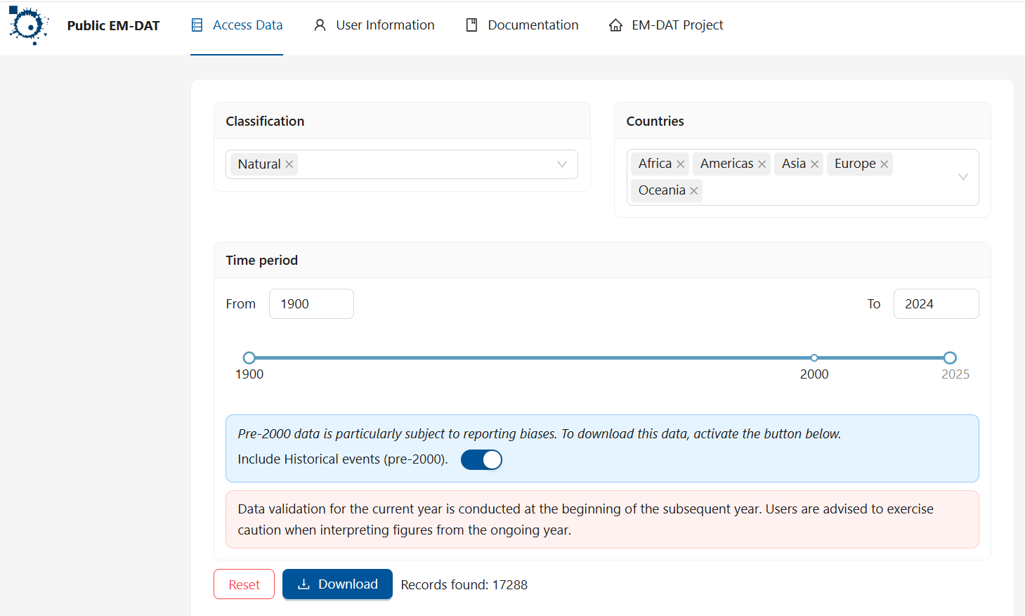
After clicking download you should find that an EXCEL workshet was downloaded. Make sure you give this worksheet a sensible name. On this occasion I named it "natural.xlsx" and, importantly, save it in the PyWork folder you created in step 1.
Step 3. Open VS Code
Open VS Code, as easy as that. Then go to Edit and Open Folder. Find the folder you create above and open that folder
Step 4. Open a script file before you start with your analysis.
A crucial part of working with Python is that you document your work by saving all the code commands you apply in either a script file (.py) or a Jupyter notebook (.ipynb).
We recommend that on most occasions (and certainly at the beginning of your coding career) you should work in Jupyter Notebook with the extension ".ipynb".
To be able to work with Jupyter notebooks you will have to add the Jupyter extension. If, when clicking on the Extension icon on the left hand side you do not see the Jupyter extension extension then type Jupyter into the Search box and follow the installation instruction. You can also look at this useful 6min YouTube video.

A Jupyter notebook allows you to save your commands (code), comments, and outputs in one document. The process that you need to follow consists of the steps outlined here:
- Create a new notebook by going to File → New File and then chose Jupyter Notebook.
- Give that file a sensible name and save it in your working directory (e.g., my_first_pywork.ipynb).
- Remember to frequently save your work (CTRL + S on windows or Cmd+S on a Mac).
Now, let's create a Jupyter Notebook file following the abovementioned steps. A Jupyter notebook basically consists of code and markdown blocks. markdown blocks, like the one in the image below, basically contain text and code blocks (see below) will contain python code. It is best to start with a markdown block in which you tell yourself what this notebook is about. Whether a block is code or markdown you can see at the bottom right of every block. You can change between the two types if you click the three dots in the top right of each block.
If you want a new block you click on either the + Code or the + Markdown button. A list with useful Jupyter notebook formatting support is available from here.
A more detailed introductory workthrough is available from ECLR.]
Step 5. Type and execute code in your file.
Somewhere underneath, into your script, type the line below. Then have your cursor in that line and either press the run button or type CTRL + ENTER.
print(5+2) # Summation
a = 5677170409**(0.5) # ** takes the power
b = a-76*1000
7
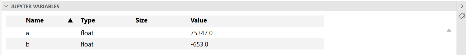
Here we created two new objects, a and b and you should be able to see these in the list of Jupyter variables.

Once you click on "Jupyter Variables" the following tab should become visible.
Comments
What are comments?
Note that the text after "#" is a comment and will be ignored by Python. YOu
Why should I write comments?
There are a number of reasons why you should be adding comments to your code. By far the most important is to communicate with your future self. Imagine you are writing code for a project which has a deadline in three weeks. However, you will have to interrupt the exciting data work for a week to finish an essay. When you return to your code in a week time you will have forgotten why you did certain things. Unless, you have added sufficient comments to your code explaining to your future self why you did certain things.
Do add comments liberally.
You should find that the variable b is now a negative number.
Step 6. Save your work
Save the file. If you are working in a jupyter workbook the file will have an ".ipynb" extension. If you work in a pure code file the extension will be ".py". The file will contain all your commands you have used in the current session and allows you to replicate what we have done in the future easily. But more importantly than replicating is that it will also document clearly what you have done.
Do make sure that the file is saved in your working directory.
Working in VS Code
There are a few more things to note as you are working in VS code. For what follows we will assume that you are working in a jupyter notebook as that is usually the best way to work as it allows you to document what you do.
Sometimes you will just want to try a line of code or execute a line of code that you know should not end up in the final code. The way how you easiest do this in this environment is that you create a new Code block in which you then write the code you want to try. Once you have done what you wanted to do you can just delete that code block.
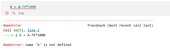
By the way, Python is case sensitive, if you try to enter b <- exp(A-76*1000) you should get an error message (Error: object 'A' not found) in the Console as R doesn't know what A is.
Task 1. Installing and Loading Python libraries.
The Python software comes with a lot of functionality as you download it to your computer. As it is an open-source software, anyone can add functionality to Python. This added functionality come in batches of code that are called "packages" or "libraries". To use any of this added functionality, you first need to install the relevant package and then activate (or load) it into your session. Once the package is activated, you can access and use the functions it contains.
Here we will use four packages, os, numpy, pandas and lets-plot
The step you will always have to do is to load the libraries into your session. Let's do that with the first three libraries.
# Import necessary libraries
import os as os # for operations at the operating system level
import pandas as pd # For data manipulation
import numpy as np # For numerical computations
Most likely you can run these lines without an error message as they are routinely pre-loaded.
The way how these libraries have been imported implies that any functionality will be addressed with a prefix. For instance, to calculate an exponential, using the exp function from the numpy library we would make the following call:
c = np.exp(4)
Using these prefixes, which are defined as you import the libraries is particularly important in case there may be functions of the same name, but from different packages.
Some packages you may need are unlikely to be installed on your computer. Let's attempt to import functionality from the lets-plot library.
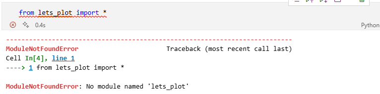
Above you can see an error message. "No module named lets_plot basically tells you that that module (or library) has not yet been installed.
Install libraries in Python.
To install a library, if needed, you need to open a terminal. Go to ""Terminal"" - ""New Terminal"" and you should see a Terminal tab at the bottom of your VS Code screen. It will show the file path to your current worksheet and then a ">". Type "pip install lets-play" and press ENTER. The computer will do its thing and download the lets-plot library. You will see a bunch of lines appear in the Terminal. The last one shoudl read something like "Successfully installed lets_plot ..."
Now you should be able to load the library into your code.
from lets_plot import * # For data visualization
LetsPlot.setup_html()
Loading a library needs doing everytime you load your script.
Key point:
Install a library: just do once
Activate a library: do it every time you need
This means that you have installed the lets-plot package this time. In future instances, there is no need to reinstall it. However, you will need to activate it as we did above every time you want to use functions from the lets-plot function.
Task 2. Import the Excel data set into Python.
Once the readxl library is activated, we can use its read_excel() function to import the "natural.xlsx" dataset. We then store the imported dataset in an object named emdat.
emdat = pd.read_excel("natural.xlsx")
What does this line of code actually do?
Reading Code
It is extremely important to be able to read code and understand what it does. This is especially true in a world where we increasingly do not have to write code from scratch but have helpers at our hand that deliver code. But you need to remember that you are the quality control and are responsible for the code doing what you want it to do.
So what does the code do?
Here we are using the assignment operator = which tells Python to define a new object, here emdat, with whatever is on the right hand side of the assignment operator. On the right and side we are using the pd.read_excel function. As it uses the prefix pd. Python knows that it can find this function in the pandas library.
Functions are the bread and butter of working in Python or any other language. Hidden behind read_excel is a lot of code that achieves a particular purpose. Usually that code needs some input variable(s). These input variables are delivered in the parentheses directly after the function name. How many and what inputs are needed depends on the function. You can find details on that by looking at the function's documentation. A straightforward way of accessing that is to go to a browser and look for "Python read_excel" which will lead you to the documentation for the read_excel function.
The input is the path to the EXCEL file we wish to import. Note that the default path used is the working directory we set previously. The function does take that EXCEL file and converts it into a dataframe (think about it as the equivalent of a spreadsheet in Python) which then can be used in Python. Once you executed this line you should see emdat when you look at the "Jupyter variables".
How to read documentation?
In the previous tab you were advised to look at the documentation for the read_excel function. When you start out working with code these documentation files can be somewhat overwhelming. Let's look at the information you can get from the documentation for the read_excel function.
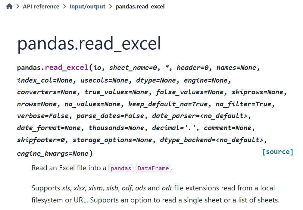
What you can see at the top of the documentation is the name of the function and a list of all the potential parameters the function will accept. It starts with "pandas.read_excel(io, ...)". To figure out what the first input is the function expects you can scroll down to the Parameters
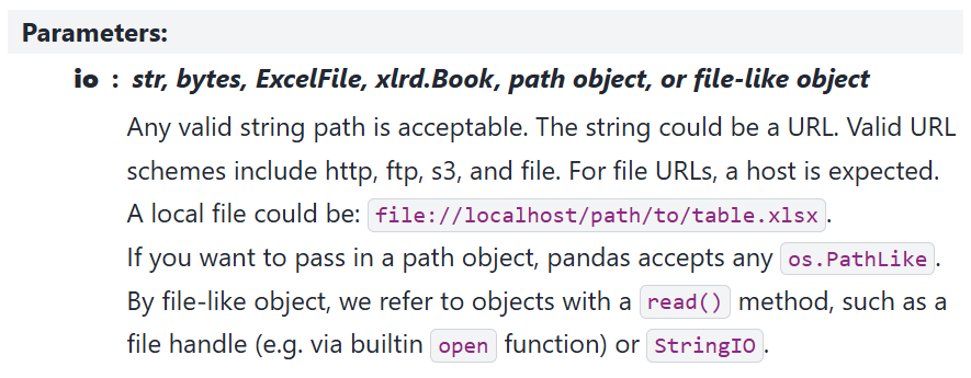
From there you can perhaps infer that what is needed is a path to a file and Python expects this to be delivered as a string object. In our above function call this is "natural.xlsx". But as you can tell, the language is quite techy. What often helps is if you scroll further down to the Examples section of the documentation. There you will for instance find the following.
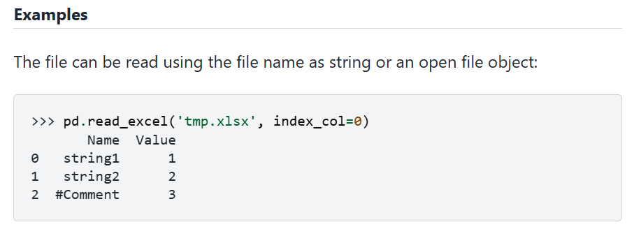
From here you can understand what is expected. In that example the file being imported is "temp.xlsx". In that example you can also see that a 2nd option is used ("index_col=0"). Let's find out what this is for. In the first image, where all parameters are listed in teh function call you can see that it says "index_col = none". This means that by default, i.e. when you do not call that parameter, it is set to "non". But what does it mean. To figure that out you go to the Parameters list to find the following entry for this parameter:
It refers to how to name the entries/rows in the dataframe. By default ("none") read_excel assumes that there are no row labels in the imported sheet and Python will automatically allocate labels 0, 1, 2, etc to the rows.
Initial data exploration
Let's explore the data. When you open the Jupyter Variables tab you can immediately see from the Environment tab that the object has 17,288 observations (or rows) and 46 variables (or columns).
If you double click on the emdat line in the variable list you can actually see the spreadsheet.
Sometimes it is useful to see a list of all the column/variable names. This is easily achieved by the following line.
emdat.columns
Index(['DisNo.', 'Historic', 'Classification Key', 'Disaster Group',
'Disaster Subgroup', 'Disaster Type', 'Disaster Subtype',
'External IDs', 'Event Name', 'ISO', 'Country', 'Subregion', 'Region',
'Location', 'Origin', 'Associated Types', 'OFDA/BHA Response', 'Appeal',
'Declaration', 'AID Contribution ('000 US$)', 'Magnitude',
'Magnitude Scale', 'Latitude', 'Longitude', 'River Basin', 'Start Year',
'Start Month', 'Start Day', 'End Year', 'End Month', 'End Day',
'Total Deaths', 'No. Injured', 'No. Affected', 'No. Homeless',
'Total Affected', 'Reconstruction Costs ('000 US$)',
'Reconstruction Costs, Adjusted ('000 US$)',
'Insured Damage ('000 US$)', 'Insured Damage, Adjusted ('000 US$)',
'Total Damage ('000 US$)', 'Total Damage, Adjusted ('000 US$)', 'CPI',
'Admin Units', 'Entry Date', 'Last Update'],
dtype='object')
Another line that achieves the same (and more) is the following:
emdat.dtypes
DisNo. object
Historic object
Classification Key object
Disaster Group object
Disaster Subgroup object
Disaster Type object
Disaster Subtype object
External IDs object
Event Name object
ISO object
Country object
Subregion object
Region object
Location object
Origin object
Associated Types object
OFDA/BHA Response object
Appeal object
Declaration object
AID Contribution ('000 US$) float64
Magnitude float64
Magnitude Scale object
Latitude float64
Longitude float64
River Basin object
Start Year int64
Start Month float64
Start Day float64
End Year int64
End Month float64
End Day float64
Total Deaths float64
No. Injured float64
No. Affected float64
No. Homeless float64
Total Affected float64
Reconstruction Costs ('000 US$) float64
Reconstruction Costs, Adjusted ('000 US$) float64
Insured Damage ('000 US$) float64
Insured Damage, Adjusted ('000 US$) float64
Total Damage ('000 US$) float64
Total Damage, Adjusted ('000 US$) float64
CPI float64
Admin Units object
Entry Date object
Last Update object
dtype: object
Here you can not only see the names but also the data types. The first variable (DisNo) is of type object which is basically a text or character variable. This variable is a unique identifier for a disaster. Most variables are of type object, float64 (any number) or int64 (natural numbers). Data types are important as there are some things you cannot do with certain variable types. For instance you couldn't multiply object variables as multiplication with text is not defined.
Some of the variable names are very long and it may be useful to shorten them.
emdat.rename(columns={"AID Contribution ('000 US$)": "AID.Contr",
"Reconstruction Costs ('000 US$)": "Rec.Cost.adj",
"Insured Damage ('000 US$)": "Ins.Damage",
"Insured Damage, Adjusted ('000 US$)": "Ins.Damage.adj",
"Total Damage ('000 US$)": "Total.Damage",
"Total Damage, Adjusted ('000 US$)": "Total.Damage.adj"},
errors="raise", inplace=True)
What does this line of code actually do?
Reading Code
Earlier we learned about functions and how they are applied. In the previous few lines you saw another important technique. On each occasion we did something with the dataframe emdat. And the way we did that was by calling the object, then a "." and then a name of a method, these were columns, dtypes and rename.
What are methods?
You can think of methods as functions which only make sense for a particular type of object, here a dataframe.
The rename method looks complicated
Applying the rename method here was indeed more complicated than applying columns or dtypes. Recall, methods are functions and some functions require additional input. To rename column names you had to tell python which columns you want to rename and then to which name. That is basically the information provided by, say "AID Contribution ('000 US$)": "AID.Contr" which gave basically the old and then the new column name.
The columns and dtypes method merely told us something about some characteristic of the dataframe emdat. The rename method however, actually changed the emdat object. However, it only does so as we set the addition al option inplace=True. If that was not set, it would have printed a new dataframe with the new columns but would not have saved the new names in emdat.
What methods are there for dataframes?
There are a lot. Too many to list here for sure. You could look at this page to see some of the most important ones or could ask ChatGPT to give you an overview of the most important methods for panda dataframes.
Let's look at a particular natural catastrophe, the one with indicator DisNo. == "2019-0209-CHN".
emdat.loc[emdat['DisNo.'] == "2019-0209-CHN"]
| DisNo. | Historic | Classification Key | Disaster Group | Disaster Subgroup | Disaster Type | Disaster Subtype | External IDs | Event Name | ISO | ... | Rec.Cost.adj | Reconstruction Costs, Adjusted ('000 US$) | Ins.Damage | Ins.Damage.adj | Total.Damage | Total.Damage.adj | CPI | Admin Units | Entry Date | Last Update | |
|---|---|---|---|---|---|---|---|---|---|---|---|---|---|---|---|---|---|---|---|---|---|
| 14815 | 2019-0209-CHN | No | nat-hyd-flo-flo | Natural | Hydrological | Flood | Flood (General) | NaN | NaN | CHN | ... | NaN | NaN | 700000.0 | 858892.0 | 6200000.0 | 7607333.0 | 81.500309 | [{"adm1_code":900,"adm1_name":"Chongqing Shi"}... | 2019-06-14 | 2023-09-25 |
1 rows × 46 columns
This is a flooding incident that happened in China in late June 2019. 300 people died and 4.5 million were affected according to the information in the database. Here is a BBC news article on this heavy rain incident.
You can learn much more about the structure of the database, how the data are collected and checked and the variable descriptions from this documentation page.
So far we haven't done any analysis on the data, but let's start to use the power of the software. Let's say you want to look at some summary statistics for some variables, for instance you are interested in how many people are affected by the natural catastrophes in the database (Total Affected).
We will now use the describe method, but only applied to the Total Affected column.
emdat['Total Affected'].describe()
count 1.280200e+04 mean 6.927568e+05 std 7.385030e+06 min 1.000000e+00 25% 7.040000e+02 50% 6.000000e+03 75% 6.000000e+04 max 3.300000e+08 Name: Total Affected, dtype: float64
You can see that the natural disasters registered here affect on average almost 700,000 people, with a max of 330 million. But almost 5000 events have no information on the number of affected people. Especially early events do not have such information.
The describe method works well for numerical variables. For categorical data a different method will give you better information.
We can also see a breakdown of the type of incidents that have been recorded. This is recorded in the Disaster Subgroup variable (for all incidents here Disaster Group == "Natural").
emdat['Disaster Subgroup'].value_counts()
Disaster Subgroup Hydrological 6897 Meteorological 5550 Geophysical 1941 Biological 1610 Climatological 1289 Extra-terrestrial 1 Name: count, dtype: int64
We find hydrological events (e.g. heavy rainfalls) to be the most common type of natural disaster.
PRACTICE
Task
Identify the Extra-terrestrial incident in the dataset and see whether you can find any related news reports.
Hint
If you wish to find a particular incident you can use the same structure of a code line as we did to display the particular event above. You will just have to change the variable name by which you filter and the value it should take accordingly.
Complete Solution
emdat.loc[emdat['Disaster Subgroup'] == "Extra-terrestrial"]
| DisNo. | Historic | Classification Key | Disaster Group | Disaster Subgroup | Disaster Type | Disaster Subtype | External IDs | Event Name | ISO | ... | Rec.Cost.adj | Reconstruction Costs, Adjusted ('000 US$) | Ins.Damage | Ins.Damage.adj | Total.Damage | Total.Damage.adj | CPI | Admin Units | Entry Date | Last Update | |
|---|---|---|---|---|---|---|---|---|---|---|---|---|---|---|---|---|---|---|---|---|---|
| 12583 | 2013-0060-RUS | No | nat-ext-imp-col | Natural | Extra-terrestrial | Impact | Collision | NaN | NaN | RUS | ... | NaN | NaN | NaN | NaN | 33000.0 | 44436.0 | 74.263729 | [{"adm1_code":2499,"adm1_name":"Chelyabinskaya... | 2014-03-21 | 2024-02-06 |
1 rows × 46 columns
Note that we did not create a new object, we merely extracted some information and displayed it.
An alternative way to achieve the same (and there are always different ways to achieve the same thing) is:
emdat.query("`Disaster Subgroup` == 'Extra-terrestrial'")
| DisNo. | Historic | Classification Key | Disaster Group | Disaster Subgroup | Disaster Type | Disaster Subtype | External IDs | Event Name | ISO | ... | Rec.Cost.adj | Reconstruction Costs, Adjusted ('000 US$) | Ins.Damage | Ins.Damage.adj | Total.Damage | Total.Damage.adj | CPI | Admin Units | Entry Date | Last Update | |
|---|---|---|---|---|---|---|---|---|---|---|---|---|---|---|---|---|---|---|---|---|---|
| 12583 | 2013-0060-RUS | No | nat-ext-imp-col | Natural | Extra-terrestrial | Impact | Collision | NaN | NaN | RUS | ... | NaN | NaN | NaN | NaN | 33000.0 | 44436.0 | 74.263729 | [{"adm1_code":2499,"adm1_name":"Chelyabinskaya... | 2014-03-21 | 2024-02-06 |
1 rows × 46 columns
Being able to access particular elements in a dataframe is a very important skill. You can discover different techniques on ECLR.
And here is a BBC article on the meteorite.
Complete the code below to extract the event.
PRACTICE
Task
Find the disaster event by which 330000000 people were affected.
Hint
The number 330000000 is the maximum number of people affected by a natural diaster in the database. Use the same technique used above.
emdat.loc[emdat[XXXX] == XXXX]
Solution check
You got it right if you get the following event:
| DisNo. | Historic | Classification Key | Disaster Group | Disaster Subgroup | Disaster Type | Disaster Subtype | External IDs | Event Name | ISO | ... | Rec.Cost.adj | Reconstruction Costs, Adjusted ('000 US$) | Ins.Damage | Ins.Damage.adj | Total.Damage | Total.Damage.adj | CPI | Admin Units | Entry Date | Last Update | |
|---|---|---|---|---|---|---|---|---|---|---|---|---|---|---|---|---|---|---|---|---|---|
| 13639 | 2015-9618-IND | No | nat-cli-dro-dro | Natural | Climatological | Drought | Drought | NaN | NaN | IND | ... | NaN | NaN | 400000.0 | 529395.0 | 3000000.0 | 3970461.0 | 75.557977 | [{"adm1_code":1485,"adm1_name":"Andhra Pradesh... | 2016-04-11 | 2024-04-09 |
1 rows × 46 columns
You should find that the code extracts event "2015-9618-IND". The natural catastrophe that affected more than 300 Mio people was a drought in the Indian subcontinent.
Simple summary statistics
The following is one fo the most common type of data analysis.
In order to better understand what type of disasters the different subgroups represent we can look at the following bit of code, which uses piping:
table_1 = emdat.groupby(['Disaster Subgroup', 'Disaster Type'])\
.agg(n=('DisNo.', 'count'), Avg_Affected=('Total Affected', 'mean'))\
.reset_index()
# the "\" at the end of the line tells python that the statement continues on the next line
print(table_1)
Disaster Subgroup Disaster Type n Avg_Affected 0 Biological Animal incident 1 5.000000e+00 1 Biological Epidemic 1514 3.851679e+04 2 Biological Infestation 95 6.404400e+05 3 Climatological Drought 796 5.504330e+06 4 Climatological Glacial lake outburst flood 5 2.951967e+04 5 Climatological Wildfire 488 5.791003e+04 6 Extra-terrestrial Impact 1 3.014910e+05 7 Geophysical Earthquake 1617 1.762719e+05 8 Geophysical Mass movement (dry) 46 1.217211e+03 9 Geophysical Volcanic activity 278 4.403567e+04 10 Hydrological Flood 6049 7.798324e+05 11 Hydrological Mass movement (wet) 848 3.781653e+04 12 Meteorological Extreme temperature 696 7.019187e+05 13 Meteorological Fog 1 NaN 14 Meteorological Storm 4853 4.267879e+05
What does this line of code actually do?
Reading Code
It is important to understand what the above operation does, or in other words it is an important skill to be able to read what a line of code does. Try to understand what the elements in that line do.
We start with the dataframe emdat and then apply a method (groupby) but then another method is appended (agg). This way of working is called method chaining (for those familiar with working in R, this is rather similar to piping).
So here it firsts groups the data by two variables and then continues to aggregate or summarise the resulting groups. Have another close look and see whether you can understand what is going on.
Where to find help?
One way to get support with this is to ask a LLM like ChatGPT to help you read that code.
Experiment with the code
A great way to understand what some code does is to experiment a little and see what happens if you change the code. A part of the code, the purpose of which is somewhat unclear, is that last method applied, reset_index().
The easiest way to figure out what this does is to leave that part of the code out and see what happens (or doesn't happen). Try that!
This is like a data production line. Just imagine how much work this would have been in Excel (although pivot tables get close to the convenience).
PRACTICE
The task
Now I want you to produce a similar table but group the data by Region and calculate the average aid received (AID.Contr) and the average total estimated damage (Total.Damage).
Hint
Copy and paste the previous table and adjust what needs adjusting.
The rename method looks complicated
here is the skeleton code:
table2 = emdat.groupby('XXXX') \
.XXXX(n=('DisNo.', 'count'),
Avg_Contribution=('XXXX', 'mean'),
Avg_Total_Damage=('XXXX', 'XXXX')) \
.XXXX()
XXXX(table2)
Complete solution
Here is the complete solution. But have you struggled enough? Struggling is an important part of the learning process.
table2 = emdat.groupby('Region') \
.agg(n=('DisNo.', 'count'),
Avg_Contribution=('AID.Contr', 'mean'),
Avg_Total_Damage=('Total.Damage', 'mean')) \
.reset_index()
print(table2)
Region n Avg_Contribution Avg_Total_Damage 0 Africa 3188 7889.918367 1.830913e+05 1 Americas 4304 24435.508380 1.251189e+06 2 Asia 6907 28062.363112 7.698964e+05 3 Europe 2174 1882.113208 6.332938e+05 4 Oceania 715 3566.204082 3.787227e+05
This is the end of Task 2, where we imported the database with natural disasters and did some initial data exploration.
Reflection
Question
Why is it so important to save your work in a file (script file or jupyter workbook)?
What are methods?
Let's compare to working in EXCEL, which is perhaps the software you would have used for such work previously. Let's imagine it is the end of the day again and you are closing down your computer. You could have done all that work in EXCEL and may have produced great tables. Next morning you get up and you realise that you actually did need to know the original variable names. Well in EXCEL you would not know anymore what they are, as you changed them. YOu would have to go back to the original datafile (perhaps even download it again). Here, we still have the original datafile and you can just go to the code where you change the names and adjust that.
Or you wanted to create summary tables using a different grouping variable. In EXCEL you would have to go through the process of creating the table again. Here, as everything is saved in a script, you just go to the line where you set the grouping variable, change it and press the Source button as that will the re-run your entire code.
Task 3: A Simple Plot Tells a Lot
Above we already presented some useful summary statistics, such as the mean or maximum for a numeric variable, or frequencies for categorical variables. However, often the best way to convey a story is to use graphs. Here we are using the extremely powerful ggplot function. This is not here to actually teach you how this works, but just to wet your appetite (you can find more detail on the graphing techniques on ECLR]).
As we are thinking about the impact of climate change there is a lot of talk about natural disasters becoming more frequent. Let us count the disasters of different types every year and then show this information as a time-series plot. This should demonstrate whether there is indeed an increasing number of natural disasters in the database.
table_3 = emdat.groupby(['Disaster Type', 'Start Year']).agg(n=('DisNo.', 'count')).reset_index()
Have a look at table_3 to understand the structure of that object.
Investigate the data
Question
Which of the following best describes the structure of table_3?
- Each Disaster.Type-Year has its own row
- Each Disaster.Type has its own row, Years are in columns
- Each Country-Disaster.Type has its own row, Years are in columns
- Each Country-Years has its own row, Disaster.Types are in columns
- Each Country-Disaster.Type-Year has its own row
Answer
Correct Answer: Each Disaster.Type-Year has its own row
The following code produces a line graph.
plot_ts = (ggplot(table_3, aes(y='n', x='Start Year', colour = 'Disaster Type')) +
geom_line())
plot_ts
What does this line of code actually do?
Reading Code
The ggplot functions allows you to build graphs in a fairly intuitive way. But, this is not really a session to learn the details of graphing in R.
But I am curious?
As you are curious, here is a quick run through of what the code does.
plot_ts =, A new object calledplot_tsis created from the code on the right hand side of=ggplot(table_3, ), tells Python to create a plot using the data intable_3, although at this stage it doesn't know yet what plot.aes(y='n', x='Start Year', colour = 'Disaster Type'), basically tells Python what should be on the axis of the plot,Start Yearon the horizontal axis (x), the number of disasters per year (n) on the vertical axis and that the data should be separated (and shown in different colours) byDisaster Type. But we still have not instructed Python what type of plot to create.+ geom_line(), this is where we instruct R to actually create a line plot with the earlier parameters (trygeom_points()to see the difference). This concludes the plot creation.plot_ts, this just instructs R to actually display the plot we saved inplot_ts
You can learn more about how to create great graphs with ggplot from this page on ECLR.
We can immediately see that some of the events have seen massive increases. However, we need to be aware that there are issues with relying on this dataset. Some of these are discussed on the data's website, in particular what they call the time bias, reflecting the insight that the increase in number of disasters may partly be driven by increased data collection.
Reconsidering the plot above it is apparent that it is on the messy side as some categories are very small and make seeing the core information more difficult. So we will filter out event types that overall small number of observations.
Let's look again at the Disaster Types and how many observations we have in each category:
emdat['Disaster Type'].value_counts()
Disaster Type Flood 6049 Storm 4853 Earthquake 1617 Epidemic 1514 Mass movement (wet) 848 Drought 796 Extreme temperature 696 Wildfire 488 Volcanic activity 278 Infestation 95 Mass movement (dry) 46 Glacial lake outburst flood 5 Fog 1 Impact 1 Animal incident 1 Name: count, dtype: int64
We want to pick the types that have more than 200 incidents in the database. What we need is a list of names of event types that meet this criterion. The following achieves that
sel_types = [ "Storm", "Flood", "Epidemic", "Volcanic activity", "Earthquake",
"Drought" , "Mass movement (wet)" ,"Wildfire", "Extreme temperature" ]
However, it is good to learn how to do this in an automatic way as these type of problems can be so big that it is impractical to do manually.
sel_types2 = emdat.groupby('Disaster Type') \
.agg(n=('DisNo.', 'count')) \
.query('n > 199') \
.index.tolist()
You can again check with ChatGPT to ensure that you understand what these steps achieved.
Why did we need a list of disaster types we want to focus on? The reason is that with that list in hand we can easily filter out the data we want to concentrate on. To do that we use the filter function, in particular we want to filter (i.e. keep) the data that relate to disaster types that are contained in sel_types2.
Run the following code
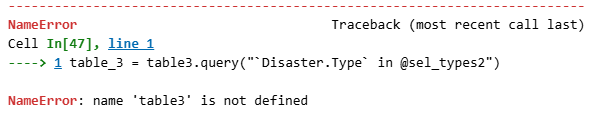
table_3 = table3.query("`Disaster Type` in @sel_types2")
When you do so you will get an error message, something like
Debugging code
What does the error message say?
Try to figure out what the problem is. The error message points at table3 as the problem. What is table3?
What are debugging strategies?
Dealing with error messages is a bread and butter activity for anyone who works with data in the way we do here. Note the following about error messages:
- Receiving error messages is normal and you CANNOT break your computer
- Errors protect you from doing unwanted things to your data
- The error messages are SOMETIMES helpful in identifying the cause of the problem
- Sometimes the error messages point at a symptom rather than the root cause of the problem. (this is in fact the case here)
Here are some tips on how to deal with error messages:
- Re-read what you typed, is it 'exactly' what you wanted? (Python is case sensitive!)
- Do the objects you refer to actually exist in the Environment?
- Re-run code one line at a time and identify line with error.
- Read error message and try to find anything that you can understand. Don't worry about the parts you don't understand – there will be lots!
Can you fix the code?
Solution
We are not giving you the correct solution here. If you follow the above advice you will be able to fix the problem.
Before this operation table_3 had 864 rows of data. If that has reduced to 802 rows then you have achieved the correct result.
Now we can re-run the graph.
plot_ts = (ggplot(table_3, aes(y='n', x='Start Year', colour = 'Disaster Type')) +
geom_line())
plot_ts
It is still slighty messy. There are two ways to certainly improve the readability of the graph. We could smooth the data series to get a more obvious picture of the time trend. We will not do this here as it will require a bit more work. Another aspect would be to only display data from 1970 onwards. It does appear as before that date the activity stays approximately constant.
Use the query method to remove all data up to 1969 and then re-plot the graph.
table_3 = table_3.XXXX("`Start Year` > XXXX")
plot_ts = (XXXX(XXXX, aes(y='XXXX', XXXX='Start Year', XXXX = 'XXXX')) +
geom_line())
plot_ts
There are perhaps still too many lines to see clearly how these different types develop. There is a fairly straightforward way to visually disentangle these.
plot_ts = plot_ts + \
facet_wrap(["Disaster Type"], nrow = 3, ncol = 3)
plot_ts
What is remarkable here, and one of the reasons why the ggplot functions are so popular, is that you can add functionality to an existing plot (here ts_plot). In particular we keep teh previous plot but do isntruct Python to split the graph into seperate plots by Disaster Type. This is what + facet_wrap(["Disaster Type"], nrow = 3, ncol = 3) does.
The two disaster types that have seen a very obvious increase are floods (green) and storms (storms), but wildfires, wet mass movements and extreme temperatures have also seen a steady increase (note that all graphs are on identical scales). All of these can plausibly be linked to climate change. The two geological events (earthquakes and volcanic eruptions) have not seen an obvious increase.
Country level emission data
It is often said that the effects of climate change do predominantly hit the countries that are not actually responsible for the bulk of the greenhouse gas (GHG) emissions that cause rising temperatures. In the disaster database we have information on which countries are affected by natural disasters only. We will now link the data from the disaster dataset with another dataset from which we can get information on GHG. Linking datasets is an extremely important activity for anyone dealing with real life data, an activity deserving a place in such an introduction.
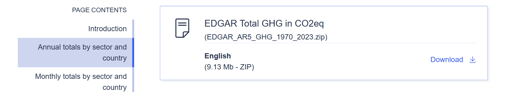
That dataset is the EDGAR dataset maintained by the European Union. We are downloading the 2024 version of the dataset, in particular the "EDGAR Total GHG in CO2eq" version.
 {width="50%"}
When you download this you will get a zip file and you should extract the contents of the zip file into your working directory. One of the files is an EXCEL file called "EDGAR_AR5_GHG_1970_2023.xlsx". Let us load this file.
edgardat = pd.read_excel("EDGAR_AR5_GHG_1970_2023.xlsx")
edgardat.head()
| Unnamed: 0 | |
|---|---|
| 0 | Conditions of use and how to cite |
| 1 | NaN |
| 2 | © European Union 2024, European Commission, Jo... |
| 3 | NaN |
| 4 | All emissions, except for CO2 emissions from f... |
This does not look like a proper datafile. What has gone wrong? Not all mistakes generate an error message. Sometimes Python will do something but it is not what we want to achieve.
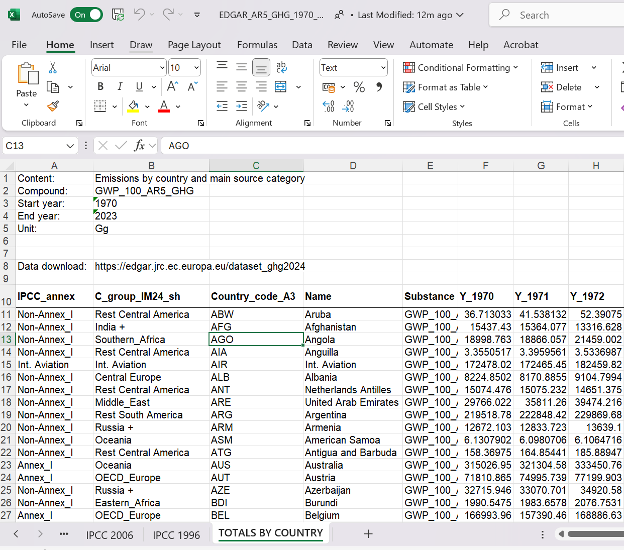
Before uploading a datafile into Python it is important to understand the structure of the datefile. Hence we should actually open the file in EXCEL and look at it to understand its structure.
 {width="50%"}
As you look at the file you will see that there are several tabs with data and by default the read_excel function imports the first. But that is not the one with the data we want. The sheet that contains the data we want to look at is called "TOTALS BY COUNTRY" (sheet_name = "TOTALS BY COUNTRY"). On that sheet we notice something else. The data sheet only starts in row 10 with the variable names. So when we import this we want to ignore the first 9 rows (skiprow = 9). We need to instruct Python to do that. Before you retry the import make sure that you close the spreadsheet.
edgardat = pd.read_excel("EDGAR_AR5_GHG_1970_2023.xlsx", sheet_name = "TOTALS BY COUNTRY", skiprows = 9)
edgardat.head()
| IPCC_annex | C_group_IM24_sh | Country_code_A3 | Name | Substance | Y_1970 | Y_1971 | Y_1972 | Y_1973 | Y_1974 | ... | Y_2014 | Y_2015 | Y_2016 | Y_2017 | Y_2018 | Y_2019 | Y_2020 | Y_2021 | Y_2022 | Y_2023 | |
|---|---|---|---|---|---|---|---|---|---|---|---|---|---|---|---|---|---|---|---|---|---|
| 0 | Non-Annex_I | Rest Central America | ABW | Aruba | GWP_100_AR5_GHG | 36.713033 | 41.538132 | 52.390750 | 57.359887 | 56.630192 | ... | 469.468414 | 490.990250 | 514.539464 | 496.140535 | 495.531919 | 588.997896 | 482.159941 | 531.201512 | 533.603088 | 561.497605 |
| 1 | Non-Annex_I | India + | AFG | Afghanistan | GWP_100_AR5_GHG | 15437.430263 | 15364.077308 | 13316.628180 | 13934.875093 | 15177.862417 | ... | 27420.132302 | 27408.331772 | 26633.998536 | 27691.927104 | 27553.281612 | 26982.776572 | 26646.320070 | 27643.074355 | 28614.071224 | 29460.052110 |
| 2 | Non-Annex_I | Southern_Africa | AGO | Angola | GWP_100_AR5_GHG | 18998.762967 | 18866.057085 | 21459.002495 | 23018.940660 | 23685.423333 | ... | 77295.699295 | 81775.030635 | 78875.889482 | 73424.409437 | 69504.638320 | 69910.831904 | 61680.081008 | 64408.994317 | 67210.841707 | 67700.756248 |
| 3 | Non-Annex_I | Rest Central America | AIA | Anguilla | GWP_100_AR5_GHG | 3.355052 | 3.395956 | 3.533699 | 3.411377 | 3.694243 | ... | 31.209941 | 31.334184 | 31.728472 | 32.475516 | 31.594224 | 30.947736 | 26.037062 | 25.224274 | 25.068398 | 26.210752 |
| 4 | Int. Aviation | Int. Aviation | AIR | Int. Aviation | GWP_100_AR5_GHG | 172478.021013 | 172465.451921 | 182459.818548 | 190296.909848 | 183162.103533 | ... | 514263.976095 | 543354.254566 | 567631.286648 | 597771.580137 | 624135.612321 | 633464.501865 | 302632.336740 | 335728.729280 | 416953.421848 | 498178.114415 |
5 rows × 59 columns
This has worked! Let's have a look at the structure of the edgardat object. We have 225 rows of data, one for each country. The real data are saved in columns which have the years in the title. So the structure is like this
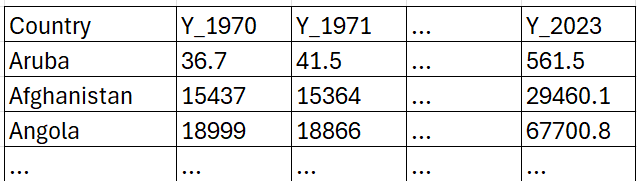
where the numbers are the CO2 equivalent GHG emissions for a particular country in a particular year.
This way of presenting data is sometimes called a wide format. It is not the best format to have your data in if you want to work in Python (or any other language). We really want the data in what is called the long format:
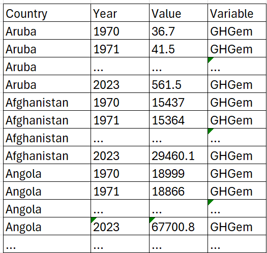
If you only keep one variable you could do without the Variable column, but with that variable you can also keep several variables in the same structure. Basically each observation (Country-Year-Variable) has its own row.
The question is then how to translate the current wide version into a long version.
# Determine which variables should stay (indic_vars) and which should become a variable
indic_vars = edgardat.columns[:5] # picks the first 5 (0 to 4) variable names
vars_to_year = edgardat.columns[5:] # picks the variable names that are years (from 6th variable to end)
# Convert wide to long format
edgardat_long = edgardat.melt(id_vars = indic_vars, value_vars = vars_to_year,
var_name='YEAR', value_name='GHG.em')
# Remove "Y_" prefix from 'YEAR' column
edgardat_long['YEAR'] = edgardat_long['YEAR'].str.replace("Y_", "", regex=False)
# Convert 'Year' column to integer
edgardat_long['YEAR'] = edgardat_long['YEAR'].astype(int)
The above did the trick! Here is not really the place to explain the above in detail. Suffice to say that this is a reasonably common operation such that applied economists will know that the function to use is called melt. However, unless you do this on a very regular basis one is unlikely to remember all the detail of how to apply this function by heart.
This is where ChatGPT (or another LLM) can become an excellent coding partner. You can check out this interaction with ChatGPT to see how a well formulated query can deliver the solution (teh solution here is slightly adjusted). As you can see from this example you will have to give ChatGPT very clear instruction which includes a clear understanding of what it is you want.
Now we have a file in which have we a measure of annual GHG emissions for all countries in all years. Among these countries we have for instance China (which is massive) but also Luxembourg (which is really small). We know that we should not really compare the GHG emissions for these two countries.
edgardat_long.query("YEAR == 2023 and Name in ['China', 'Luxembourg']")[["Name", "YEAR", "GHG.em"]]
| Name | YEAR | GHG.em | |
|---|---|---|---|
| 11962 | China | 2023 | 1.594399e+07 |
| 12044 | Luxembourg | 2023 | 7.860933e+03 |
Unsurprisingly China's emissions are much much larger. When dealing with issues like this we will compare per-capita statistics, i.e. we want to compare CO2 emissions per person living in a country. In order to be able to do that we first have to import population data for the countries we have.
Annual population data are available from various sources. The "WorldBank_population.csv" file contains such data, from the World Bank. Let's import these. As this is a csv file you cannot use read_excel to import this file. Try and figure out which function will import this file.
popdat = pd.XXXX("WorldBank_population.csv")
popdat.head()
| Country Name | Country Code | Indicator Name | Indicator Code | 1960 | 1961 | 1962 | 1963 | 1964 | 1965 | ... | 2015 | 2016 | 2017 | 2018 | 2019 | 2020 | 2021 | 2022 | 2023 | 2024 | |
|---|---|---|---|---|---|---|---|---|---|---|---|---|---|---|---|---|---|---|---|---|---|
| 0 | Aruba | ABW | Population, total | SP.POP.TOTL | 54922.0 | 55578.0 | 56320.0 | 57002.0 | 57619.0 | 58190.0 | ... | 107906.0 | 108727.0 | 108735.0 | 108908.0 | 109203.0 | 108587.0 | 107700.0 | 107310.0 | 107359.0 | 107624.0 |
| 1 | Africa Eastern and Southern | AFE | Population, total | SP.POP.TOTL | 130075728.0 | 133534923.0 | 137171659.0 | 140945536.0 | 144904094.0 | 149033472.0 | ... | 607123269.0 | 623369401.0 | 640058741.0 | 657801085.0 | 675950189.0 | 694446100.0 | 713090928.0 | 731821393.0 | 750503764.0 | 769294618.0 |
| 2 | Afghanistan | AFG | Population, total | SP.POP.TOTL | 9035043.0 | 9214083.0 | 9404406.0 | 9604487.0 | 9814318.0 | 10036008.0 | ... | 33831764.0 | 34700612.0 | 35688935.0 | 36743039.0 | 37856121.0 | 39068979.0 | 40000412.0 | 40578842.0 | 41454761.0 | 42647492.0 |
| 3 | Africa Western and Central | AFW | Population, total | SP.POP.TOTL | 97630925.0 | 99706674.0 | 101854756.0 | 104089175.0 | 106388440.0 | 108772632.0 | ... | 418127845.0 | 429454743.0 | 440882906.0 | 452195915.0 | 463365429.0 | 474569351.0 | 485920997.0 | 497387180.0 | 509398589.0 | 521764076.0 |
| 4 | Angola | AGO | Population, total | SP.POP.TOTL | 5231654.0 | 5301583.0 | 5354310.0 | 5408320.0 | 5464187.0 | 5521981.0 | ... | 28157798.0 | 29183070.0 | 30234839.0 | 31297155.0 | 32375632.0 | 33451132.0 | 34532429.0 | 35635029.0 | 36749906.0 | 37885849.0 |
5 rows × 69 columns
This is another dataset in wide format (international institutions love data in wide format). Use the same approach as above to turn this dataset into a new object (popdat_long) which presents the data in long format. Complete the following code to achieve this.
# Determine which variables should stay and which should become a variable
indic_vars = popdat.columns[:XXXX]
vars_to_year = popdat.XXXX[XXXX:]
# Convert wide to long format
popdat_long = popdat.XXXX(XXXX = indic_vars, XXXX = XXXX,
XXXX = 'YEAR', XXXX = 'Population')
# Convert 'YEAR' column to integer
XXXX['XXXX'] = XXXX['XXXX'].astype(XXXX)
popdat_long.head()
Solution
Struggle first
The key to learning coding is to learn to struggle. So give it a go. That means trying things out, trying to understand error messages, googling and perhaps even asking your favourite LLM.
Hint
Go back to the previous translation of a wide to a long format dataframe and try and understand the role of indic_vars and vars_to_year. This is the key to understanding what is going on.
Also try and understand why the str.replace is not needed.
Solution
# Determine which variables should stay and which should become a variable
indic_vars = popdat.columns[:4] # picks the first 4 (0 to 3) variable names
vars_to_year = popdat.columns[4:] # picks the variable names that are years (from 5th variable to end)
# Convert wide to long format
popdat_long = popdat.melt(id_vars = indic_vars, value_vars = vars_to_year,
var_name='YEAR', value_name='Population')
# Convert 'Year' column to integer
popdat_long['YEAR'] = popdat_long['YEAR'].astype(int)
popdat_long.head()
| Country Name | Country Code | Indicator Name | Indicator Code | YEAR | Population | |
|---|---|---|---|---|---|---|
| 0 | Aruba | ABW | Population, total | SP.POP.TOTL | 1960 | 54922.0 |
| 1 | Africa Eastern and Southern | AFE | Population, total | SP.POP.TOTL | 1960 | 130075728.0 |
| 2 | Afghanistan | AFG | Population, total | SP.POP.TOTL | 1960 | 9035043.0 |
| 3 | Africa Western and Central | AFW | Population, total | SP.POP.TOTL | 1960 | 97630925.0 |
| 4 | Angola | AGO | Population, total | SP.POP.TOTL | 1960 | 5231654.0 |
In order to calculate per-capita emissions we now need to bring the population and GHG emission data together. What we will do is to merge the population data into the edgar_long dataset and once we have done that we can calculate the per-capita emissions. Before we apply the merge function we strip popdat_long down to the two variables on the basis of which we will merge ("Country.Code" and "Year") and the variable which we want to merge into edgardat_long, i.e. "pop".
popdat_long = popdat_long[["Country Code", "YEAR", "Population"]]
Now we can merge this dataframe into edgardat_long.
# Merge popdat_long into edgardat_long
edgardat_long = edgardat_long.merge(popdat_long,
left_on=['Country_code_A3', 'YEAR'],
right_on=['Country Code', 'YEAR'],
how='inner')
# Drop the redundant 'Country Code' column after merging
edgardat_long = edgardat_long.drop(columns=['Country Code'])
# Display the first few rows of the merged dataframe
edgardat_long.head()
| IPCC_annex | C_group_IM24_sh | Country_code_A3 | Name | Substance | YEAR | GHG.em | Population | |
|---|---|---|---|---|---|---|---|---|
| 0 | Non-Annex_I | Rest Central America | ABW | Aruba | GWP_100_AR5_GHG | 1970 | 36.713033 | 58950.0 |
| 1 | Non-Annex_I | India + | AFG | Afghanistan | GWP_100_AR5_GHG | 1970 | 15437.430263 | 11290128.0 |
| 2 | Non-Annex_I | Southern_Africa | AGO | Angola | GWP_100_AR5_GHG | 1970 | 18998.762967 | 5852788.0 |
| 3 | Non-Annex_I | Central Europe | ALB | Albania | GWP_100_AR5_GHG | 1970 | 8224.850191 | 2135479.0 |
| 4 | Non-Annex_I | Middle_East | ARE | United Arab Emirates | GWP_100_AR5_GHG | 1970 | 29766.021550 | 286536.0 |
You will see that in edgardat_long we now also have the Population variable. The way we used the merge method was that we added what was in popdat_long to the edgardat_long. it only kept those country-year observations for which we have population data (check ?merge to see in the help function how you could change that).
Now we can calculate the per capita GHG emissions. The data in the variable GHG.em are measured in the unit Gg, or Giga grams, which is equivalent to $10^9$ grams = 1000 tonnes. The new GHG.em.pc variable we will use the unit Tonnes per person.
edgardat_long['GHG.em.pc'] = 1000 * edgardat_long['GHG.em'] / edgardat_long['Population']
Now we can compare the GHG emissions of China and Luxembourg
edgardat_long.query("YEAR == 2023 and Name in ['China', 'Luxembourg']")[["Name", "YEAR", "GHG.em", "GHG.em.pc"]]
| Name | YEAR | GHG.em | GHG.em.pc | |
|---|---|---|---|---|
| 10793 | China | 2023 | 1.594399e+07 | 11.302101 |
| 10870 | Luxembourg | 2023 | 7.860933e+03 | 11.795587 |
As it turns out, they are very similar.
Check your calculations
Why should I check calculations?
When you do such calculations you should always check that the results are actually plausible and you havn't done any mistake. This is especially important when you are manipulating units of measurement as we did here.
Once you are confiident that the calculations are correct you can move on and forget about this calculation.
How do I check calculations?
An easy way to check the calculation we did here is to go to Google or your preferred LLM and check whether the above is about right. For instance ask what is the current GHG emission per capita in Luxembourg. It turns out that our calculation is in the correct ballpark!
You can also use a calculator or a spreadsheet to check the calculation for one or two cases.
Do natural disasters happen predominantly in poor countries?
In fact the question we will really ask is whether natural disasters happen predominantly in countries that are not responsible for large GHG emissions.
Let's think what we would want to look at. In the end we will want to look at a scatter plot which has the following axes
- Average GHG emissions per capita between 1970 to date. This we can get by using the data we have in
edgardat_longand averaging across all years by country. - We need a measure of whether climate change is affecting countries more or less. Some countries are, through their geographical location, more exposed to natural disasters. E.g. countries in the Caribbean will be more exposed to storms than central European countries. We therefore should calculate a change in exposure to natural disasters. It is acknowledged that the effects of climate change have been increasing over the last few decades, as global temperatures have increased. So one way we can calculate an increased exposure to natural disasters is to calculate say the growth rate of storms (or any climate related events) from the 70s (1970 to 1979) to the the last ten years of data available (2014-2023).
Avererage GHG emissions per capita
So let's calculate these.
country_info = edgardat_long.groupby(['Country_code_A3', 'Name'])\
.agg(avg_GHG_em_pc=('GHG.em.pc', 'mean'))\
.reset_index()
We also change the name of the Country_Code_A3 variable in country_info to ISO which then matches the variable name of the three letter country code we get from the emdat data.
The following code has two errors. You will have to identify them before you can execute this line.
country_info.rename(Columns={"Country_code_A3": ISO}, inplace=True)
Solution
Solution strategies
You could compare the code to a previous time we applied the rename method to a dataframe and attempt to adjust that code.
Sometimes it is good to run the code even if you know that it is faulty. The error messages produced may well give you important hints. The error messages you are likely to receive are
- "NameError: name 'ISO' is not defined"
- "TypeError: DataFrame.rename() got an unexpected keyword argument 'Columns'. Did you mean 'columns'?"
You will only receieve one of them first.
Solution
country_info.rename(columns={"Country_code_A3": "ISO"}, inplace=True)
Don't forget the inplace=True option, otherwise the new name will not be saved in country_info.
Check afterwards by running country_info.columns in the Console to confirm that the Country code variable is now named ISO.
Growth in natural disasters
We basically need to calculate two measures of exposure to natural disasters (those that can potentially be linked to the effects of climate change), a measure for the 70s, the base measure, and then a recent measure.
Let us look back at the information in the emdat database, by looking at a particular event. In particular we need to understand how events that affect multiple countries are recorded. To investigate this we will attempt to identify Hurricane Sandy (Wikipedia entry to Hurricane Sandy) which, in late October 2012 affected several countries in the Carribean and then the US. So let's filter by what we know.
test = emdat.query("`Start Year` == 2012 & `Start Month` == 10 & `Disaster Subgroup` == 'Meteorological'")
There are 14 events selected and if you look at the data you will see that in the Event Name variable there is actually an indication which events are related to Hurricane Sandy. So we can actually filter on that.
test = emdat.query("`Event Name` == 'Hurricane Sandy'")[['DisNo.', 'Event Name', 'ISO', 'Country', 'Start Year', 'Start Month', 'Start Day']]
print(test)
DisNo. Event Name ISO Country \
12402 2012-0410-BHS Hurricane Sandy BHS Bahamas
12403 2012-0410-CUB Hurricane Sandy CUB Cuba
12404 2012-0410-DOM Hurricane Sandy DOM Dominican Republic
12405 2012-0410-HTI Hurricane Sandy HTI Haiti
12406 2012-0410-JAM Hurricane Sandy JAM Jamaica
12407 2012-0410-USA Hurricane Sandy USA United States of America
Start Year Start Month Start Day
12402 2012 10.0 24.0
12403 2012 10.0 22.0
12404 2012 10.0 24.0
12405 2012 10.0 24.0
12406 2012 10.0 24.0
12407 2012 10.0 28.0
As you can see, for each affected country we get a separate event. This will greatly facilitate our measure of exposure to climate change as we are calculating country level exposures.
Understanding your data
Why is it important?
What we did here is perhaps one of the most important activities an applied economist or data scientist will ever have to do. UNDERSTAND THE DATA. This will involve looking at particular data examples. Investigate what variables are available, understand what the unit of observation is, understand the sample of data available to you, be knowledgeable about the limitations the data come with.
How do I do that?
There is no general recipe to do that. You will have to be curious and ask critical questions. Here we knew that we should be able to find a particular event (Hurricane Sandy) in the data and then we went to find it in the data. If you see how something you know is represented in the data then this can be a great path to understanding the data.
On top of that looking at summary statistics and graphical representations is often a great path to improved data understanding.
In order to calculate exposure we begin by calculating the number of events that affected a particular country between 1970 and 1979. But we will only count the events that could potentially be explained by climate change, i.e. those in the following Disaster.Subgroup: Climatological, Hydrological and Meteorological.
sel_dis_types = ["Climatological", "Hydrological", "Meteorological"]
Country_info_dis_base = emdat.query("`Disaster Subgroup` in @sel_dis_types & `Start Year` > 1969 & `Start Year` < 1980")\
.groupby('ISO')\
.agg(base=('DisNo.', 'count'))\
.reset_index()
Note, we are explicitly not claiming that any individual event here is the result of climate change. We can see that we have counts of events for 124 countries. That means that a good number of countries did not experience any disasters.
You could quite rightly ask why we don't just take the disaster count in countries in 1970 and compare that to 2023. Why do we need to calculate averages?
The reason is that disasters are a lumpy occurrence. There can be a particular year with many bad storms being followed by a year without. And then it matters whether 1970 was one or the other. Climate measures should always be taken over longer periods and not just a year.
And in fact we could also consider aggregating regionally across countries.
Now we do the same but for the most recent years (2014-2023).
Country_info_dis_recent = emdat.XXXX("`Disaster Subgroup` in @sel_dis_types & `Start Year` > XXXX & `XXXX` < XXXX")\
.groupby(['ISO','Region'])\
.agg(recent=('DisNo.', 'XXXX'))\
.reset_index()
You will know that you got it right if Country_info_dis_recent has 201 observations and 3 variables and the first few rows look like this.
Country_info_dis_recent.head()
| ISO | Region | recent | |
|---|---|---|---|
| 0 | AFG | Asia | 49 |
| 1 | AGO | Africa | 20 |
| 2 | AIA | Americas | 1 |
| 3 | ALB | Europe | 9 |
| 4 | ARE | Asia | 1 |
Note, that here we also added Region as a grouping variable. This isn't really necessary, but it will add Region to Country.info.dis.recent and we will make good use of that variable as we plot the data.
The first indication that the number of disasters has increased is that we are now counting events for more than 200 countries, however, do remember that a recency bias is one of the biases potentially contained in the database. Another bias may be that in general the reporting in more advanced countries is better. Being conscious of that point we will still proceed by merging the two data objects we just created. We will merge these variables into the country_info database in which we already saved the avg.GHG.em.pc variable.
country_info = country_info.merge(Country_info_dis_base, on='ISO', how='left')
What does this code actually do?
merge architecture
The way the merge function is used here is as a method. We take one dataframe (country_info) and apply the merge method. That means that we are merging another dataframe (here `Country_info_dis_base) into that datframe.
merge options
The merge function does require inputs, at the very least the two dataframes that require merging (here only one in addition to the one to which the method is applied). The on option indicates which are variable(s) that are being matched from both dataframes. Here that is the ISO variable, meaning we match on countries. You could actually leave this at its default (by not listing the on option in the call of the method) in which case python woudl find the variables that have the same name and matchon that. But to make the code more readable it is best to add this option.
The second important input option is the how option. Here we chose how = 'left'. What this does is to make sure that the result of the merge action retains all the rows which were in country_info. If it finds a matching row in Country_info_dis_base it will add the respective info of the new variables. Check out the other possible settings for the how option are.
How to find details?
You should start by looking at the function documentation which you can access by searching for "pandas merge". Look at the options (and their default values) and also look at the examples at the bottom of the documentation to see what effect the different options have. Of course you could also go to your favourite LLM and ask it to explain the different options.
And now we add the recent variable to country.info dataframe. Use exactly the same settings as in the merge we just performed.
country_info = country_info.merge(XXXX)
Solution
Try yourself
As always you should first try this yourself. Follow the previous example. Copy and paste the code and try and adjust it.
Solution
country_info = country_info.merge(Country_info_dis_recent, on='ISO', how='left')
Check your result
You got the result right if the first few rows look like this:
country_info.head
<bound method NDFrame.head of ISO Name avg_GHG_em_pc base Region recent 0 ABW Aruba 3.355769 NaN NaN NaN 1 AFG Afghanistan 0.938111 5.0 Asia 49.0 2 AGO Angola 3.096369 NaN Africa 20.0 3 ALB Albania 3.212663 NaN Europe 9.0 4 ARE United Arab Emirates 47.590699 NaN Asia 1.0 .. ... ... ... ... ... ... 198 WSM Samoa 1.930623 NaN Oceania 2.0 199 YEM Yemen 1.245250 NaN Asia 21.0 200 ZAF South Africa 10.341670 3.0 Africa 36.0 201 ZMB Zambia 1.877387 1.0 Africa 10.0 202 ZWE Zimbabwe 2.737963 1.0 Africa 13.0 [203 rows x 6 columns]>
And now we can calculate a growth rate of number of incidents (nat.dis.gr) and the log difference (nat.dis.dlog). The latter can be preferable for a number of reasons.
# Add the growth rate of natural disasters
country_info['nat.dis.gr'] = (country_info['recent'] - country_info['base']) / country_info['base']
# Add the log difference of natural disasters
country_info['nat.dis.dlog'] = np.log(country_info['recent']) - np.log(country_info['base'])
You should again look at your calculations and ensure that the everything looks sensible.
sel_countries = ["China", "Luxembourg", "Mexico"]
country_info.query("Name in @sel_countries")
| ISO | Name | avg_GHG_em_pc | base | Region | recent | nat.dis.gr | nat.dis.dlog | |
|---|---|---|---|---|---|---|---|---|
| 34 | CHN | China | 5.415383 | 4.0 | Asia | 197.0 | 48.250000 | 3.896909 |
| 111 | LUX | Luxembourg | 29.809649 | NaN | Europe | 4.0 | NaN | NaN |
| 118 | MEX | Mexico | 5.399160 | 13.0 | Americas | 54.0 | 3.153846 | 1.424035 |
There are a number of things we can learn from this.
- For countries which did not report any natural disasters in the base period we can not calculate a growth rate (any growth from 0 would be infinite growth). Luxembourg is an example in case here.
- In the case of Mexico we counted 13 natural disasters in the base period and 54 in the recent period. The latter number is 315% larger than the former. This growth is recorded as 3.15.
- In the case of China we see that in the base period only 4 natural disasters were recorded in the database. This seems an implausibly low number and reminds us that at the time information in China was tightly controlled. One result of this may be that the international recording of natural disasters has not been happening at the same level of openness and accuracy with which it has been done for the more recent period. This serves as a reminder that you always have to think about the data quality.
Data Quality
Why does it matter?
Data quality should always be considered as a potential issue. Problems could arise from different issues
- Different efforts tro record certain things (this could be differences across countries or time), this is certainly a potential issue here
- Definitions may be different across time and space
- Improving quality of some measuring equipment
This will matter if important decisions are based on an analysis based on potentially dodgy data.
How should I communicate this?
In the first instance you have to be open about your doubts when you communicate any analysis based on these data. Often you can do very little to change the data and openness is the best approach. Let the user of your analysis decide whether the data quality means that your analysis should not be trusted.
As we may be somewhat dubious especially with the event count in the base period there is a number of numerical precautions you could make. Perhaps we could move the base period to the 80s, or when we look at increased exposure we may rely more on the log difference (nat.dis.dlog). For the actual growth rate the dubious number, the base period, does go into the denominator and that has a massive numerical influence. The log difference is less susceptible to eratic movements in the base period.
Despite the above reservations we are now plotting the scatter plot we indicated earlier we wanted to plot.
country_info.columns
Index(['ISO', 'Name', 'avg_GHG_em_pc', 'base', 'Region', 'recent',
'nat.dis.gr', 'nat.dis.dlog'],
dtype='object')
plot_scatter = ggplot(country_info, aes(y='nat.dis.gr', x='avg_GHG_em_pc', colour = 'Region')) +\
geom_point()
plot_scatter
There are a number of issues with this plot, let's fix them:
plot_scatter = plot_scatter + \
xlim(0,30) + \
labs(x = "p.c. GHG emissions", y = "Increase in nat. dis. exposure", \
title ="GHG emissions and natural disasters")
plot_scatter
There does seem to be some negative correlation. The countries with the highest GHG emissions do not have the largest exposure to increases in natural disasters. The largest increases seem to come from countries with lowest GHG emissions. But do recall that we ought to be somewhat careful about the growth data, especially if they come from countries with potentially dubious base year data. Looking at the log difference will protect us to a certain degree.
plot_scatter2 = ggplot(country_info, aes(y='nat.dis.dlog', x='avg_GHG_em_pc', colour = 'Region')) + \
geom_point() + \
xlim(0,30) + \
labs(x = "p.c. GHG emissions", y = "Increase in nat. dis. exposure", \
title ="GHG emissions and natural disasters")
plot_scatter2
Now we can see that there is no obvious relationship between the two variables. But do note that almost all countries here experience a significant increase in exposure to natural disasters that can potentially be linked to climate change, irrespective of how much they contribute to the problem.
So the above analysis does not say that there are no effects of climate change. In contrast we do observe a global increase in the number of natural disasters. But they seem to be hitting high and low polluters in to a similar extend.
What the analysis here cannot show is that poorer countries (usually the ones with lower emissions) are less equipped to actually deal with the consequences of increased natural disasters. But that would be a new and equally interesting analysis.
End of session
Before you leave VS Code you need to save your code file. That means that tomorrow you can just come back open the notebook and continue to work.
Conclusion
In this workthrough we presented a graphical representation of the relationship between GHG emission behaviour and increased exposure to natural disasters at a country level. In the process of producing this graphical evidence we did a number of common tasks for any data scientist.
- Finding relevant data
- Importing data into R
- Cleaning data
- Producing summary statistics
- Producing graphical representations of data
- Calculating new variables
- Merging data from different datasets
We also learned a number of things about working as an applied economist or data scientist.
- Always save your work in script or notebook files!
- Commenting your code will save your future self a lot of time
- Error messages are part of the daily life
- Fixing errors in code is super important
- Some errors stop the code from running but other errors are not so obvious (hence you always need to test whether you have actually achieved what you wanted to achieve)
- Using the help function is important
- Using Google, ChatGPT or other LLMs can help you out, but to use them you need to know quite a bit and you need to ask well-formulated questions
Solution
Solution strategies
text 0
Solution?
text 1
The rename method looks complicated
text 2
What methods are there for dataframes?
text 3